Content from Introduction and Experimental Planning Considerations for RNA-Seq

---

Last updated on 2024-08-16 | Edit this page

Estimated time: 70 minutes

Overview

Questions

• What is RNA-Seq?
• What data are we using?
• Why is this experiment important?

Objectives

• Learn about the history and the current status of gene expression research.
• How do we design useful RNA-Seq experiments?
• Understand the data set through metadata.

RNA Sequencing Overview

What is RNA-Seq?

RNA Sequencing (RNA-Seq) is a powerful technology used to analyze the transcriptome of a sample by sequencing RNA molecules.

Key Applications: - Gene expression profiling - Differential Gene Expression - Discovery of novel transcripts - Analysis of alternative splicing events - Study of non-coding RNAs

RNA Sequencing

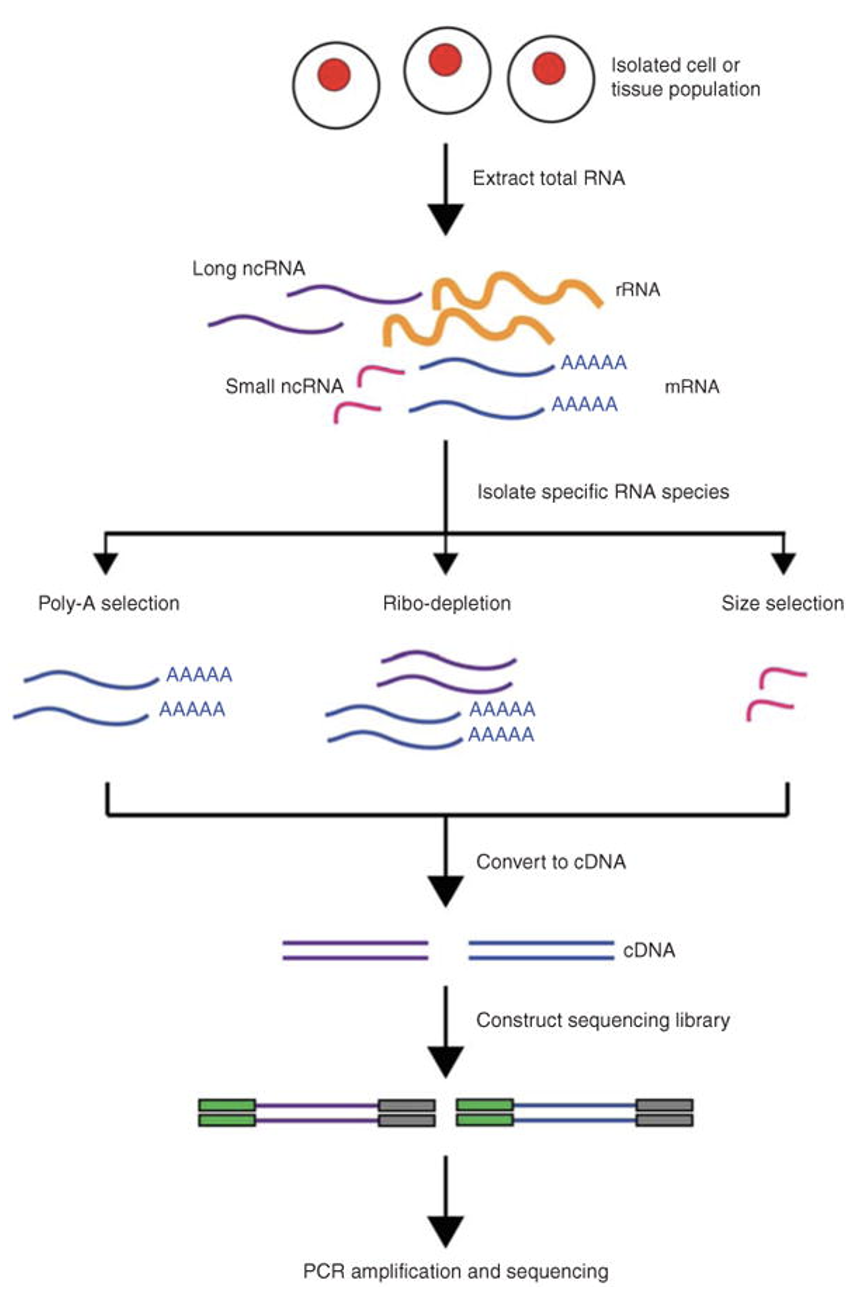
RNA-Seq Workflow

• RNA Extraction: RNA is extracted from the biological material of choice (e.g., cells, tissues).
• Library Preparation: The RNA is converted to complementary DNA (cDNA) by reverse transcription
• Adapter Ligation: Sequencing adaptors are ligated to the ends of the cDNA fragments.
• Sequencing: Following amplification, the RNA-Seq library is ready for sequencing.

RNA-Seq Workflow Diagram

Sequencing on Illumina Platforms

Illumina sequencing uses Sequencing by Synthesis (SBS) technology where nucleotides are incorporated into a growing DNA strand and the sequence is determined by the order of incorporation.

Key Illumina Platforms:

MiSeq: Older, still sometimes used for RNA-Seq or amplicon sequencing NovaSeq: High-throughput suitable for large-scale studies NextSeq: Flexible, ideal for smaller labs

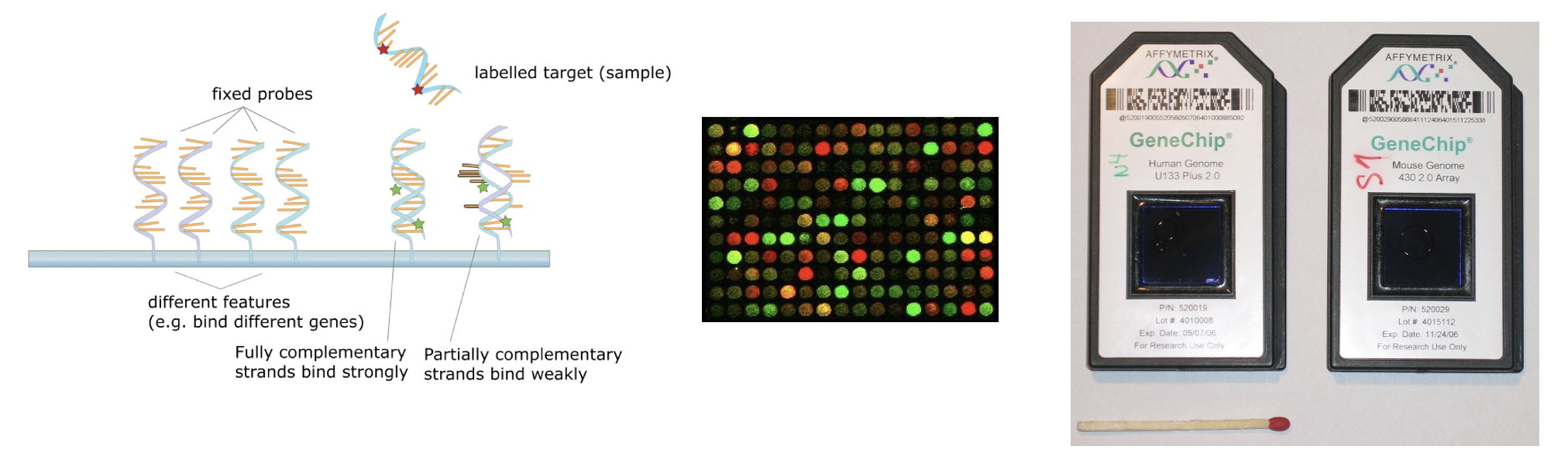
DNA MicroArray (Older Technology)

• DNA microarrays can simultaneously measure the expression level of thousands of genes within a particular mRNA sample
• The key physicochemical process involved in microarrays is DNA hybridization. Two DNA strands hybridize if they are complementary to each other, according to the Watson-Crick rules (A-T, C-G)
• mRNA is extracted from tissues or cells, reversed-transcribed and labeled with a dye (usually fluorescent), and hybridized on the array
• The next step is to generate an image using laser-induced fluorescent imaging
• The principle behind the quantification of expression levels is that the amount of fluorescence measured at each sequence-specific location is directly proportional to the amount of mRNA with complementary sequence present in the sample analyzed (relative not absolute expression)

MicroArray

MicroArray vs RNA-Seq

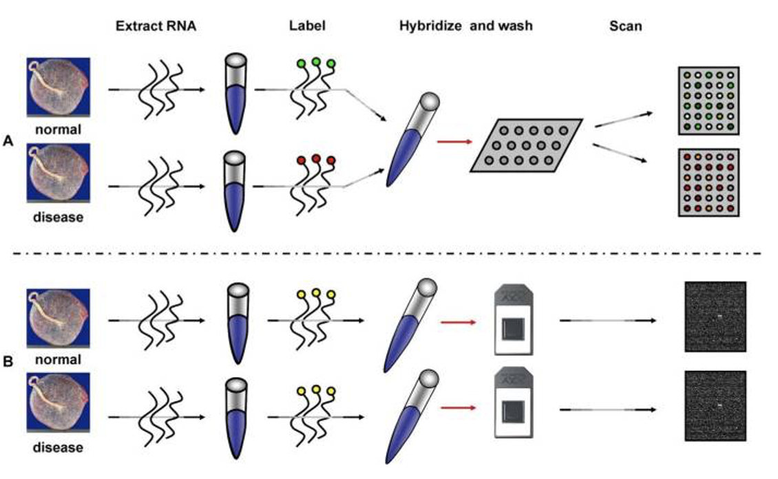
• The upper panel illustrates the two channel technology while the lower panel illustrates the single channel technology.
• The experiment is designed to compare the mRNA expression between two conditions( normal vs. disease). mRNA is extracted. In the top panel, the normal and disease mRNA are labeled with two different dyes, mixed and then hybridized on the same array. After washing, the array is scanned at two different wavelengths to yield two images
• In the bottom panel B (single channel), each sample is labeled with the same fluorescent dye, but independently hybridized on different arrays.
• Affymetrix GeneChip: oligonucleotide, single-channel array
• Terminology: “probe” is the nucleotide sequence that is attached to the microarray surface. “target” in microarray experiments refers to what is hybridized to the probes.

RNA-Seq Advantages

Unlike microarrays, RNA-Seq provides a more comprehensive view of the transcriptome, including novel transcripts and alternative splicing events. The output is typically in the form of FASTQ files, exactly like the ones we have been working with so far.

Fastq File Format

• Location on Cluster: /project/PI-groupname/project_name/
• Filenames:
  • L1_R1_CCAAT_XXX.fastq
  • L1_R2_CCAAT_XXX.fastq

Fastq format

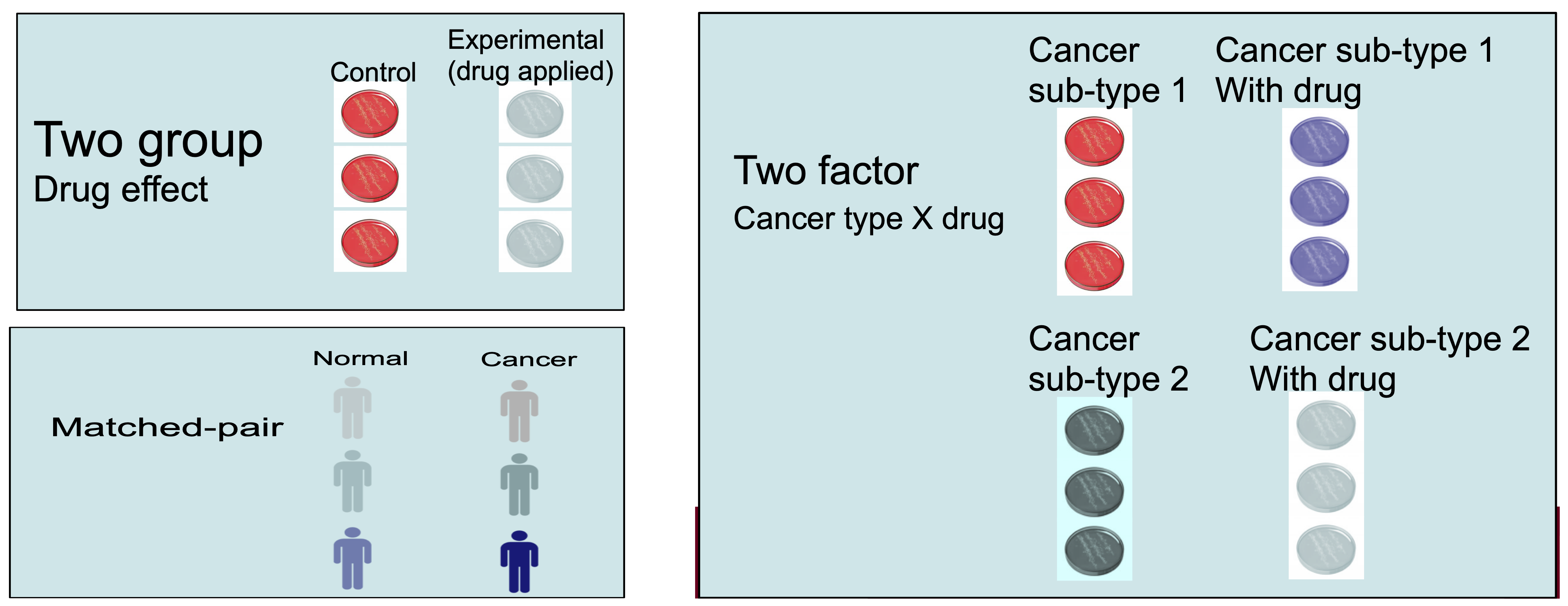
RNA-Seq Experimental Planning

---

Thoughtful experimental design is the foundation of a successful RNA-Seq study, leading to robust and reproducible results. Proper experimental design ensures that the data generated is reliable, reproducible, and has the signal strength to draw meaningful biological results. Key aspects include selecting appropriate replicates, collecting detailed metadata, and considering sources of variability.

Metadata in RNA-Seq

• Metadata refers to the descriptive information about samples.

• This includes biological details (e.g., tissue type, cell type, condition, treatment) and technical details such as library prep method, sequencing platform, sequencing depth, and sequencing batch.

• Detailed metadata is essential for understanding and interpreting the RNA-Seq data.

• Proper metadata annotation allows for better reproducibility and data sharing.

• Example:

  • Consider a case-control study, where we are interested in changes in gene expression in treated vs. untreated cells. Treatment can refer to different growth conditions, disease vs. normal, treated with a drug or vehicle.
  • Metadata should include the treatment type, dosage, duration, cell line, and batch number.

Example Metadata Table

Sample_ID	Condition	Treatment	Time_Point	Tissue_Type	Batch	Sequencing_Run	Library_Prep_Kit	RNA_Concentration (ng/µL)
Sample_01	Control	None	0 hours	Liver	1	Run_01	Kit_A	200
Sample_02	Treated	Drug_X	6 hours	Liver	1	Run_01	Kit_A	210
Sample_03	Control	None	12 hours	Liver	1	Run_02	Kit_B	190
Sample_04	Treated	Drug_X	24 hours	Liver	2	Run_02	Kit_B	220
Sample_05	Control	None	0 hours	Heart	2	Run_03	Kit_A	230
Sample_06	Treated	Drug_X	6 hours	Heart	2	Run_03	Kit_A	215
Sample_07	Control	None	12 hours	Heart	3	Run_04	Kit_B	205
Sample_08	Treated	Drug_X	24 hours	Heart	3	Run_04	Kit_B	225

Metadata Explanation

• Sample_ID: A unique identifier for each sample.
• Condition: Indicates the experimental condition (e.g., control, treated).
• Treatment: Details of any treatment applied to the samples (e.g., Drug_X).
• Time_Point: The time point at which the sample was collected.
• Tissue_Type: The type of tissue from which the sample was extracted.
• Batch: The batch number indicating when the samples were processed.
• Sequencing_Run: The specific sequencing run in which the sample was sequenced.
• Library_Prep_Kit: The kit used for sequencing library preparation.
• RNA_Concentration: The concentration of RNA in the sample, which is important for assessing sample quality.

Biological and Technical Replicates

• Biological replicates are independent samples from the same experimental condition.

• They capture natural biological variability, which is crucial for generalizing results.

• These replicates are crucially needed for downstream statistical analysis.

• Technical replicates involve repeating the same sample processing steps (e.g., sequencing, library prep) to assess technical variability (instrument measurement noise).

• Replicates increase the reliability of your findings by allowing for statistical analysis.

• It is highly recommended to generate at least 3 biological replicates per condition to ensure sufficient statistical power for detecting differential expression.

Randomization and Block Design

• Randomization refers to randomly assigning samples to different experimental conditions or processing orders to minimize bias.

• Randomization helps to evenly distribute confounding factors (e.g., time of day, machine variability) across all experimental conditions.

• Block design is a strategy where samples are grouped into blocks that share a common characteristic (e.g., batch) to control for known sources of variability.

• Example:

  • If you are processing samples in different batches, you can randomize the order of sample processing within each batch to avoid systematic errors.

Experimental Design

Confounding Factors and Batch Effects

• Confounding factors are variables that can influence the outcome of the experiment without being of direct interest (e.g., technician handling, machine type, sequencing center).
• Batch effects are unwanted variations that arise from differences in sample processing or sequencing batches.
• Confounding factors and batch effects can obscure the true biological signals in the data.
• Design stage: Include batch as a factor in your experimental design.
• Analysis stage: Apply batch effect correction methods, such as ComBat or include batch as a covariate in the statistical model.

Challenge

Based on the information metadata.csv in ~/itcga_workshop/metadata/, can you answer the following questions?

1. How many different fastq files do we have?
2. How many rows and how many columns are in this data?
3. How many CXCL12-treated samples do we have? Note that each sample has more than one associated file.

Show me the solution

1. 36 files
2. 36 rows, 6 columns
3. Three samples (S4,S5,S6), each with four files (PE = R1 & R2 on lane = L1 & L2)

Key Points

• RNA-Seq is a powerful tool for understanding differences in gene expression in various experiments.
• There are many ways to analyze these data, and we will show you one of them.
• It is important to record and understand your experiment’s metadata.
• Carefully plan your experiment to account for potential sources of variability.
• Use appropriate numbers of biological replicates and consider technical replicates where necessary.
• Randomize sample processing and use block designs to minimize bias.
• Address batch effects during both the design and analysis stages.

Content from Assessing Read Quality

---

Last updated on 2025-01-03 | Edit this page

Estimated time: 50 minutes

Overview

Questions

• How can I describe the quality of my data?

Objectives

• Explain how a FASTQ file encodes per-base quality scores.
• Interpret a FastQC plot summarizing per-base quality across all reads.
• Use for loops to automate operations on multiple files.

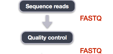
Bioinformatic workflows

---

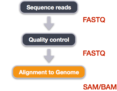
When working with high-throughput sequencing data, the raw reads you get off of the sequencer will need to pass through a number of different tools in order to generate your final desired output. The execution of this set of tools in a specified order is commonly referred to as a workflow or a pipeline.

An example of the workflow we will be using for our transcriptome (also known as RNA-Seq or gene expression) analysis is provided below with a brief description of each step.

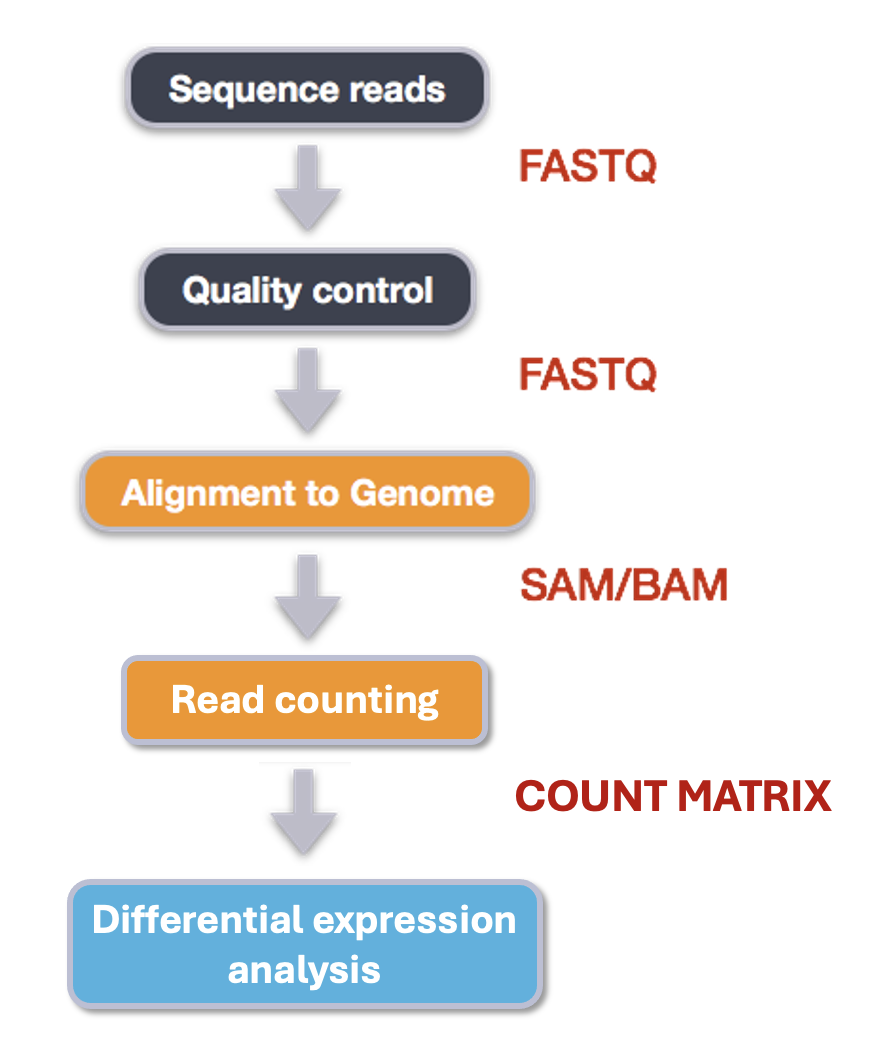
1. Quality control - Assessing quality using FastQC
2. Quality control - Trimming and/or filtering reads (if necessary)
3. Align reads to reference genome
4. Count the number of reads at each gene
5. Analyze differences in gene expression across samples

These workflows in bioinformatics adopt a plug-and-play approach in that the output of one tool can be easily used as input to another tool without any extensive configuration. Having standards for data formats is what makes this feasible. Standards ensure that data is stored in a way that is generally accepted and agreed upon within the community. The tools that are used to analyze data at different stages of the workflow are therefore built under the assumption that the data will be provided in a specific format.

Starting with data

---

Our data are three samples from an experiment on the conversion of fibroblasts to myofibroblasts, Patalano et al. 2018. There are two known signalling proteins involved in the conversion of prostate fibroblasts to myofibroblasts: TBF-beta and CXCL12. These proteins both affect which genes get transcribed in cells, but they act on different pathways and do not affect all of the same genes as each other.

In this experiment, fibroblasts were treated with either TGF-beta, CXCL12, or a control (termed ‘vehicle’). The first letter of each sample name corresponds to the treatment (eg. the samples treated with TGF-beta begin with T and the vehicle controls begin with a V). For each sample, we have one file with all the forward reads and one file with all the reverse reads.

Quality control

---

We will now assess the quality of the sequence reads contained in our fastq files.

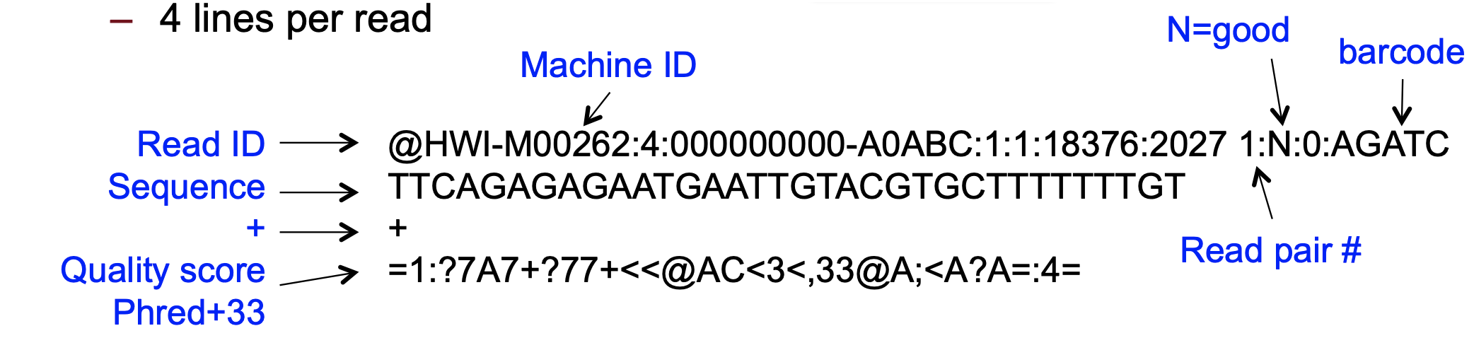
Details on the FASTQ format

Although it looks complicated (and it is), we can understand the fastq format with a little decoding. Some rules about the format include…

Line	Description
1	Always begins with ‘@’ and then information about the read
2	The actual DNA sequence
3	Always begins with a ‘+’ and sometimes the same info in line 1
4	Has a string of characters which represent the quality scores; must have same number of characters as line 2

We can view the first complete read in one of the files our dataset by using head to look at the first four lines.

BASH

$ head -n 4 C1_S4_L001_R2_001_downsampled.fastq

OUTPUT

@D00345:37:HBATBADXX:1:1214:3724:1975 2:N:0:GCCAAT
NNNNNNNAATCNTTNCAANTCTCTTGCAAGGTNCCCTGGTTGNGAAAATAC
+
#######22:@#2:#22>#2@3=?=<?@??<<#0:;=??>>?#0-=??>>=

Line 4 shows the quality for each nucleotide in the read. Quality is interpreted as the probability of an incorrect base call (e.g. 1 in 10) or, equivalently, the base call accuracy (e.g. 90%). To make it possible to line up each individual nucleotide with its quality score, the numerical score is converted into a code where each individual character represents the numerical quality score for an individual nucleotide. For example, in the line above, the quality score line is:

OUTPUT

#######22:@#2:#22>#2@3=?=<?@??<<#0:;=??>>?#0-=??>>=

The numerical value assigned to each of these characters depends on the sequencing platform that generated the reads. The sequencing machine used to generate our data uses the standard Sanger quality PHRED score encoding, using Illumina version 1.8 onwards. Each character is assigned a quality score between 0 and 41 as shown in the chart below.

OUTPUT

Quality encoding: !"#$%&'()*+,-./0123456789:;<=>?@ABCDEFGHIJ
                   |         |         |         |         |
Quality score:    01........11........21........31........41

Each quality score represents the probability that the corresponding nucleotide call is incorrect. This quality score is logarithmically based, so a quality score of 10 reflects a base call accuracy of 90%, but a quality score of 20 reflects a base call accuracy of 99%. These probability values are the results from the base calling algorithm and depend on how much signal was captured for the base incorporation.

Looking back at our read:

OUTPUT

@D00345:37:HBATBADXX:1:1214:3724:1975 2:N:0:GCCAAT
NNNNNNNAATCNTTNCAANTCTCTTGCAAGGTNCCCTGGTTGNGAAAATAC
+
#######22:@#2:#22>#2@3=?=<?@??<<#0:;=??>>?#0-=??>>=

We can now see that there is a range of quality scores, but that the start of the sequence is very poor (# = a quality score of 2).

Exercise

What is the last read in the V1_S1_L001_R1_001_downsampled.fastq file? How confident are you in this read?

Show me the solution

BASH

$ tail -n 4 V1_S1_L001_R1_001_downsampled.fastq

OUTPUT

@D00345:37:HBATBADXX:1:1206:21030:101413 1:N:0:CGATGT
GTTACTCGACCGAAGTCTTCACTATGCATCACAACTCAAGATTANNNTANA
+
@@@FDDFFHGDHHIGFH@@GGHGIIIIIGGDCEGGFHHGFGGAH###--#-

This read has higher quality quality overall than the first read that we looked at, but still has a range of quality scores, including low-quality bases at the end. We will look at variations in position-based quality in just a moment.

At this point, let’s validate that all the relevant tools are installed. If you are using the Chimera then these should be pre-installed, but you’ll need to load some modules.

Why do we need to load modules? Chimera is a shared resource used by many different people working on many different types of projects. Not everybody needs to be able to use the same programs as each other, and if we had every program loaded at the same time it would potentially slow the chimera down and lead to conflicts between programs. Let’s take a look at how many different modules exist on the chimera:

BASH

$ module avail

That was a lot!! Remember you can use clear to calm your terminal down. Let’s look for just the module we need, by typing its name after module avail.

BASH

$ module avail fastqc

----------------------- /share/apps/modulefiles/modules ------------------------
   fastqc-0.11.9-gcc-10.2.0-osi6pqc (L)

  Where:
   L:  Module is loaded

Use "module spider" to find all possible modules and extensions.
Use "module keyword key1 key2 ..." to search for all possible modules matching
any of the "keys".

If FastQC is not installed then you would expect to see an error like:

$ module avail fastqc
No module(s) or extension(s) found!
Use "module spider" to find all possible modules and extensions.
Use "module keyword key1 key2 ..." to search for all possible modules matching
any of the "keys".

If this happens check with chimera’s manager Jeff Dusenberry before trying to install it.

Now let’s load the FastQC module:

BASH

$ module load fastqc-0.11.9-gcc-10.2.0-osi6pqc

Assessing quality using FastQC

In real life, you will not be assessing the quality of your reads by visually inspecting your FASTQ files. Rather, you will be using a software program to assess read quality and filter out poor quality reads. We will first use a program called FastQC to visualize the quality of our reads. Later in our workflow, we will use another program to filter out poor quality reads.

FastQC has a number of features which can give you a quick impression of any problems your data may have, so you can take these issues into consideration before moving forward with your analyses. Rather than looking at quality scores for each individual read, FastQC looks at quality collectively across all reads within a sample. The image below shows one FastQC-generated plot that indicates a very high quality sample:

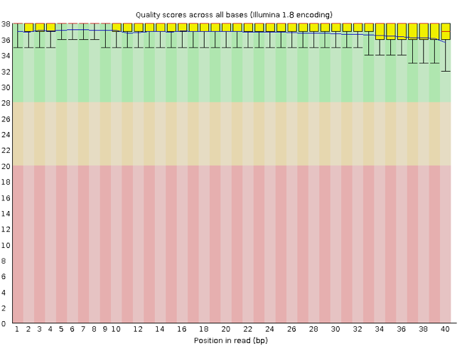
The x-axis displays the base position in the read, and the y-axis shows quality scores. In this example, the sample contains reads that are 40 bp long. This is much shorter than the reads we are working with in our workflow. For each position, there is a box-and-whisker plot showing the distribution of quality scores for all reads at that position. The horizontal red line indicates the median quality score and the yellow box shows the 1st to 3rd quartile range. This means that 50% of reads have a quality score that falls within the range of the yellow box at that position. The whiskers show the absolute range, which covers the lowest (0th quartile) to highest (4th quartile) values.

For each position in this sample, the quality values do not drop much lower than 32. This is a high quality score. The plot background is also color-coded to identify good (green), acceptable (yellow), and bad (red) quality scores.

Now let’s take a look at a quality plot on the other end of the spectrum.

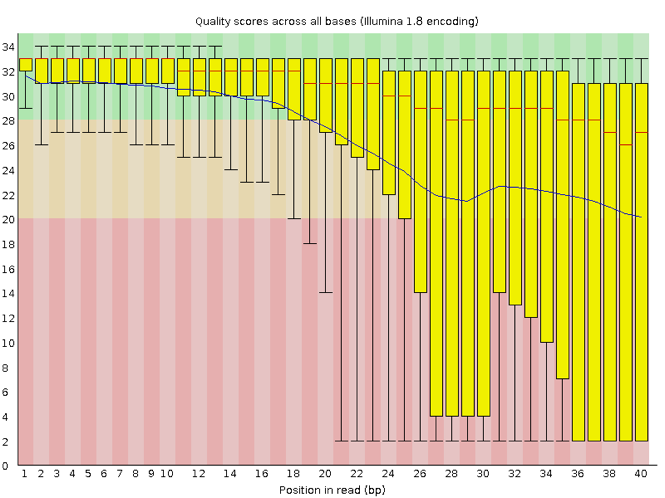
Here, we see positions within the read in which the boxes span a much wider range. Also, quality scores drop quite low into the “bad” range, particularly on the tail end of the reads. The FastQC tool produces several other diagnostic plots to assess sample quality, in addition to the one plotted above.

Running FastQC

We will now assess the quality of the reads that we downloaded. First, make sure you are still in the new untrimmed_fastq directory inside of your project’s data directory. Note that you may have named this directory something different.

BASH

$ cd ~/1_project/data/untrimmed_fastq/

Exercise

How big are the files? (Hint: Look at the options for the ls command to see how to show file sizes.)

Show me the solution

BASH

$ ls -l -h

OUTPUT

-rw-rw-r-- 1 alice.palmer001 alice.palmer001 133M Aug  7 00:54 C1_S4_L001_R1_001_downsampled.fastq
-rw-rw-r-- 1 alice.palmer001 alice.palmer001 133M Aug  7 00:54 C1_S4_L001_R2_001_downsampled.fastq
-rw-rw-r-- 1 alice.palmer001 alice.palmer001 126M Aug  7 00:55 T1_S7_L001_R1_001_downsampled.fastq
-rw-rw-r-- 1 alice.palmer001 alice.palmer001 126M Aug  7 00:55 T1_S7_L001_R2_001_downsampled.fastq
-rw-rw-r-- 1 alice.palmer001 alice.palmer001 146M Aug  7 00:55 V1_S1_L001_R1_001_downsampled.fastq
-rw-rw-r-- 1 alice.palmer001 alice.palmer001 146M Aug  7 00:55 V1_S1_L001_R2_001_downsampled.fastq

There are six FASTQ files ranging from 126M (1246B) to 1465M.

FastQC can accept multiple file names as input, and on both zipped and unzipped files, so we can use the *.fastq wildcard to run FastQC on all of the FASTQ files in this directory.

BASH

$ fastqc *.fastq

You will see an automatically updating output message telling you the progress of the analysis. It will start like this:

OUTPUT

Started analysis of C1_S4_L001_R1_001_downsampled.fastq
Approx 5% complete for C1_S4_L001_R1_001_downsampled.fastq
Approx 10% complete for C1_S4_L001_R1_001_downsampled.fastq
Approx 15% complete for C1_S4_L001_R1_001_downsampled.fastq
Approx 20% complete for C1_S4_L001_R1_001_downsampled.fastq
Approx 25% complete for C1_S4_L001_R1_001_downsampled.fastq
Approx 30% complete for C1_S4_L001_R1_001_downsampled.fastq
Approx 35% complete for C1_S4_L001_R1_001_downsampled.fastq
Approx 40% complete for C1_S4_L001_R1_001_downsampled.fastq
Approx 45% complete for C1_S4_L001_R1_001_downsampled.fastq
Approx 50% complete for C1_S4_L001_R1_001_downsampled.fastq

In total, it should take about thirty seconds for FastQC to run on all six of our FASTQ files. When the analysis completes, your prompt will return. So your screen will look something like this:

OUTPUT

Approx 60% complete for V1_S1_L001_R2_001_downsampled.fastq
Approx 65% complete for V1_S1_L001_R2_001_downsampled.fastq
Approx 70% complete for V1_S1_L001_R2_001_downsampled.fastq
Approx 75% complete for V1_S1_L001_R2_001_downsampled.fastq
Approx 80% complete for V1_S1_L001_R2_001_downsampled.fastq
Approx 85% complete for V1_S1_L001_R2_001_downsampled.fastq
Approx 90% complete for V1_S1_L001_R2_001_downsampled.fastq
Approx 95% complete for V1_S1_L001_R2_001_downsampled.fastq
Analysis complete for V1_S1_L001_R2_001_downsampled.fastq
$

Exercise

We did this directly on the command line, and it worked pretty quickly (in part because we only have six files that have been downsampled to only 5% of the original files). Usually for a task like this we will want to use a slurm script. Turn your fastqc command into a script and run it using sbatch.

Hint: You’ll need to load the module within the script and include sbatch options.

Show me the solution

BASH

$ nano fastqc.sh

#!/bin/bash

#SBATCH --job-name=fastqc # you can give your job a name
#SBATCH --nodes 1 # the number of processors or tasks
#SBATCH --cpus-per-task=2
#SBATCH --account=itcga # our account
#SBATCH --reservation=ITCGA2025 # this gives us special access during the workshop
#SBATCH --time=1:00:00 # the maximum time for the job
#SBATCH --mem=4gb # the amount of RAM
#SBATCH --partition=itcga # the specific server in chimera we are using
#SBATCH --error=%x-%A.err   # a filename to save error messages into
#SBATCH --output=%x-%A.out  # a filename to save any printed output into

# module load
module load fastqc-0.11.9-gcc-10.2.0-osi6pqc

# run fastqc
fastqc *.fastq

BASH

$ sbatch fastqc.sh

The FastQC program has created several new files within our data/untrimmed_fastq/ directory.

BASH

$ ls

OUTPUT

C1_S4_L001_R1_001_downsampled.fastq
C1_S4_L001_R1_001_downsampled_fastqc.html
C1_S4_L001_R1_001_downsampled_fastqc.zip
C1_S4_L001_R2_001_downsampled.fastq
C1_S4_L001_R2_001_downsampled_fastqc.html
C1_S4_L001_R2_001_downsampled_fastqc.zip
T1_S7_L001_R1_001_downsampled.fastq
T1_S7_L001_R1_001_downsampled_fastqc.html
T1_S7_L001_R1_001_downsampled_fastqc.zip
T1_S7_L001_R2_001_downsampled.fastq
T1_S7_L001_R2_001_downsampled_fastqc.html
T1_S7_L001_R2_001_downsampled_fastqc.zip
V1_S1_L001_R1_001_downsampled.fastq
V1_S1_L001_R1_001_downsampled_fastqc.html
V1_S1_L001_R1_001_downsampled_fastqc.zip
V1_S1_L001_R2_001_downsampled.fastq
V1_S1_L001_R2_001_downsampled_fastqc.html
V1_S1_L001_R2_001_downsampled_fastqc.zip

For each input FASTQ file, FastQC has created a .zip file and a .html file. The .zip file extension indicates that this is actually a compressed set of multiple output files. We will be working with these output files soon. The .html file is a stable webpage displaying the summary report for each of our samples.

We want to keep our data files and our results files separate, so we will move these output files into a new directory within our results/ directory.

BASH

$ mkdir -p ~/1_project/results/fastqc_untrimmed_reads
$ mv *.zip ~/1_project/results/fastqc_untrimmed_reads/
$ mv *.html ~/1_project/results/fastqc_untrimmed_reads/

Now we can navigate into this results directory and do some closer inspection of our output files.

BASH

$ cd ~/1_project/results/fastqc_untrimmed_reads/

Viewing the FastQC results

If we were working on our local computers, we would be able to look at each of these HTML files by opening them in a web browser.

However, these files are currently sitting on chimera, where our local computer can not see them. And, since we are only logging into the chimera via the command line, it does not have any web browser setup to display these files either.

So the easiest way to look at these webpage summary reports will be to transfer them to our local computers (i.e. your laptop).

To transfer a file from a remote server to our own machines, we will use scp, which we learned in the introduction to bash lessons.

First we will make a new directory on our computer to store the HTML files we are transferring. Let’s put it on our desktop for now. Open a new tab in your terminal program (you can use the pull down menu at the top of your screen or the Cmd+t keyboard shortcut) and type:

BASH

$ mkdir -p ~/Desktop/fastqc_html

Now we can transfer our HTML files to our local computer using scp. Remember to replace the username with your own!

BASH

$ scp your.UMB.username@chimera.umb.edu:/itcgastorage/share_home/your.UMB.username/itcga_workshop/untrimmed_fastq/fastqc_untrimmed_reads/*.html ~/Desktop/fastqc_html

Note on using zsh

If you are using zsh instead of bash (macOS for example changed the default recently to zsh), it is likely that a no matches found error will be displayed. The reason for this is that the wildcard (“*”) is not correctly interpreted. To fix this problem the wildcard needs to be escaped with a “\”:

BASH

$ scp your.UMB.username@chimera.umb.edu:/itcgastorage/share_home/your.UMB.username/itcga_workshop/untrimmed_fastq/fastqc_untrimmed_reads/\*.html ~/Desktop/fastqc_html

Alternatively, you can put the whole path into quotation marks:

BASH

$ scp "your.UMB.username@chimera.umb.edu:/itcgastorage/share_home/your.UMB.username/itcga_workshop/untrimmed_fastq/fastqc_untrimmed_reads/*.html" ~/Desktop/fastqc_html

The second part starts with a : and then gives the absolute path of the files you want to transfer from your remote computer. Do not forget the :. We used a wildcard (*.html) to indicate that we want all of the HTML files.

The third part of the command gives the absolute path of the location you want to put the files. This is on your local computer and is the directory we just created ~/Desktop/fastqc_html.

You should see a status output like this:

OUTPUT

your.UMB.username@chimera.umb.edu's password:
C1_S4_L001_R1_001_downsampled_fastqc.html     100%  626KB   7.4MB/s   00:00
C1_S4_L001_R2_001_downsampled_fastqc.html     100%  627KB   9.1MB/s   00:00
T1_S7_L001_R1_001_downsampled_fastqc.html     100%  629KB  10.9MB/s   00:00
T1_S7_L001_R2_001_downsampled_fastqc.html     100%  626KB   8.4MB/s   00:00
V1_S1_L001_R1_001_downsampled_fastqc.html     100%  627KB  10.3MB/s   00:00
V1_S1_L001_R2_001_downsampled_fastqc.html     100%  630KB  14.5MB/s   00:00 

Now we can go to our new directory and open the 6 HTML files.

Depending on your system, you should be able to select and open them all at once via a right click menu in your file browser.

Exercise

Discuss your results with a neighbor. Which sample(s) looks the best in terms of per base sequence quality? Which sample(s) look the worst?

Show me the solution

All of the reads contain usable data, but the quality decreases toward the beginning and end of the reads.

Decoding the other FastQC outputs

We have now looked at quite a few “Per base sequence quality” FastQC graphs, but there are nine other graphs that we have not talked about! Below we have provided a brief overview of interpretations for each of these plots. For more information, please see the FastQC documentation here

• Per tile sequence quality: the machines that perform sequencing are divided into tiles. This plot displays patterns in base quality along these tiles. Consistently low scores are often found around the edges, but hot spots can also occur in the middle if an air bubble was introduced at some point during the run.
• Per sequence quality scores: a density plot of quality for all reads at all positions. This plot shows what quality scores are most common.
• Per base sequence content: plots the proportion of each base position over all of the reads. Typically, we expect to see each base roughly 25% of the time at each position, but this often fails at the beginning or end of the read due to quality or adapter content.
• Per sequence GC content: a density plot of average GC content in each of the reads.
• Per base N content: the percent of times that ‘N’ occurs at a position in all reads. If there is an increase at a particular position, this might indicate that something went wrong during sequencing.
• Sequence Length Distribution: the distribution of sequence lengths of all reads in the file. If the data is raw, there is often on sharp peak, however if the reads have been trimmed, there may be a distribution of shorter lengths.
• Sequence Duplication Levels: A distribution of duplicated sequences. In sequencing, we expect most reads to only occur once. If some sequences are occurring more than once, it might indicate enrichment bias (e.g. from PCR). If the samples are high coverage (or RNA-seq or amplicon), this might not be true.
• Overrepresented sequences: A list of sequences that occur more frequently than would be expected by chance.
• Adapter Content: a graph indicating where adapater sequences occur in the reads.
• K-mer Content: a graph showing any sequences which may show a positional bias within the reads.

Working with the FastQC text output

Now that we have looked at our HTML reports to get a feel for the data, let’s look more closely at the other output files. Go back to the tab in your terminal program that is connected to the chimera (the tab label will start with your.UMB.username@chimerahead) and make sure you are in our results subdirectory.

BASH

$ cd ~/1_project/results/fastqc_untrimmed_reads/
$ ls

OUTPUT

C1_S4_L001_R1_001_downsampled_fastqc.html
C1_S4_L001_R1_001_downsampled_fastqc.zip
C1_S4_L001_R2_001_downsampled_fastqc.html
C1_S4_L001_R2_001_downsampled_fastqc.zip
T1_S7_L001_R1_001_downsampled_fastqc.html
T1_S7_L001_R1_001_downsampled_fastqc.zip
T1_S7_L001_R2_001_downsampled_fastqc.html
T1_S7_L001_R2_001_downsampled_fastqc.zip
V1_S1_L001_R1_001_downsampled_fastqc.html
V1_S1_L001_R1_001_downsampled_fastqc.zip
V1_S1_L001_R2_001_downsampled_fastqc.html
V1_S1_L001_R2_001_downsampled_fastqc.zip

Our .zip files are compressed files. They each contain multiple different types of output files for a single input FASTQ file. To view the contents of a .zip file, we can use the program unzip to decompress these files. Let’s try doing them all at once using a wildcard.

BASH

$ unzip *.zip

OUTPUT

Archive:  C1_S4_L001_R1_001_downsampled_fastqc.zip
caution: filename not matched:  C1_S4_L001_R2_001_downsampled_fastqc.zip
caution: filename not matched:  T1_S7_L001_R1_001_downsampled_fastqc.zip
caution: filename not matched:  T1_S7_L001_R2_001_downsampled_fastqc.zip
caution: filename not matched:  V1_S1_L001_R1_001_downsampled_fastqc.zip
caution: filename not matched:  V1_S1_L001_R2_001_downsampled_fastqc.zip

This did not work. We unzipped the first file and then got a warning message for each of the other .zip files. This is because unzip expects to get only one zip file as input. We could go through and unzip each file one at a time, but this is very time consuming and error-prone. Someday you may have 500 files to unzip!

A more efficient way is to use a for loop like we learned in the bash lessons to iterate through all of our .zip files. Let’s see what that looks like and then we will discuss what we are doing with each line of our loop.

BASH

$ for filename in *.zip
> do
> unzip $filename
> done

In this example, the input is six filenames (one filename for each of our .zip files).Each time the loop iterates, it will assign a file name to the variable filename and run the unzip command. The first time through the loop, $filename is C1_S4_L001_R1_001_downsampled_fastqc.zip. The interpreter runs the command unzip on C1_S4_L001_R1_001_downsampled_fastqc.zip. For the second iteration, $filename becomes C1_S4_L001_R2_001_downsampled_fastqc.zip. This time, the shell runs unzip on C1_S4_L001_R2_001_downsampled_fastqc.zip. It then repeats this process for the four other .zip files in our directory.

When we run our for loop, you will see output that starts like this:

OUTPUT

Archive:  C1_S4_L001_R1_001_downsampled_fastqc.zip
   creating: C1_S4_L001_R1_001_downsampled_fastqc/
   creating: C1_S4_L001_R1_001_downsampled_fastqc/Icons/
   creating: C1_S4_L001_R1_001_downsampled_fastqc/Images/
  inflating: C1_S4_L001_R1_001_downsampled_fastqc/Icons/fastqc_icon.png
  inflating: C1_S4_L001_R1_001_downsampled_fastqc/Icons/warning.png
  inflating: C1_S4_L001_R1_001_downsampled_fastqc/Icons/error.png
  inflating: C1_S4_L001_R1_001_downsampled_fastqc/Icons/tick.png
  inflating: C1_S4_L001_R1_001_downsampled_fastqc/summary.txt
  inflating: C1_S4_L001_R1_001_downsampled_fastqc/Images/per_base_quality.png
  inflating: C1_S4_L001_R1_001_downsampled_fastqc/Images/per_tile_quality.png
  inflating: C1_S4_L001_R1_001_downsampled_fastqc/Images/per_sequence_quality.png
  inflating: C1_S4_L001_R1_001_downsampled_fastqc/Images/per_base_sequence_content.png
  inflating: C1_S4_L001_R1_001_downsampled_fastqc/Images/per_sequence_gc_content.png
  inflating: C1_S4_L001_R1_001_downsampled_fastqc/Images/per_base_n_content.png
  inflating: C1_S4_L001_R1_001_downsampled_fastqc/Images/sequence_length_distribution.png
  inflating: C1_S4_L001_R1_001_downsampled_fastqc/Images/duplication_levels.png
  inflating: C1_S4_L001_R1_001_downsampled_fastqc/Images/adapter_content.png
  inflating: C1_S4_L001_R1_001_downsampled_fastqc/fastqc_report.html
  inflating: C1_S4_L001_R1_001_downsampled_fastqc/fastqc_data.txt
  inflating: C1_S4_L001_R1_001_downsampled_fastqc/fastqc.fo
Archive:  C1_S4_L001_R2_001_downsampled_fastqc.zip
   creating: C1_S4_L001_R2_001_downsampled_fastqc/
   creating: C1_S4_L001_R2_001_downsampled_fastqc/Icons/
   creating: C1_S4_L001_R2_001_downsampled_fastqc/Images/
  inflating: C1_S4_L001_R2_001_downsampled_fastqc/Icons/fastqc_icon.png
  inflating: C1_S4_L001_R2_001_downsampled_fastqc/Icons/warning.png
  inflating: C1_S4_L001_R2_001_downsampled_fastqc/Icons/error.png
  inflating: C1_S4_L001_R2_001_downsampled_fastqc/Icons/tick.png
  inflating: C1_S4_L001_R2_001_downsampled_fastqc/summary.txt
  inflating: C1_S4_L001_R2_001_downsampled_fastqc/Images/per_base_quality.png
  inflating: C1_S4_L001_R2_001_downsampled_fastqc/Images/per_tile_quality.png
  inflating: C1_S4_L001_R2_001_downsampled_fastqc/Images/per_sequence_quality.png
  inflating: C1_S4_L001_R2_001_downsampled_fastqc/Images/per_base_sequence_content.png
  inflating: C1_S4_L001_R2_001_downsampled_fastqc/Images/per_sequence_gc_content.png
  inflating: C1_S4_L001_R2_001_downsampled_fastqc/Images/per_base_n_content.png
  inflating: C1_S4_L001_R2_001_downsampled_fastqc/Images/sequence_length_distribution.png
  inflating: C1_S4_L001_R2_001_downsampled_fastqc/Images/duplication_levels.png 

The unzip program is decompressing the .zip files and creating a new directory (with subdirectories) for each of our samples, to store all of the different output that is produced by FastQC. There are a lot of files here. The one we are going to focus on is the summary.txt file.

If you list the files in our directory now you will see:

C1_S4_L001_R1_001_downsampled_fastqc
C1_S4_L001_R1_001_downsampled_fastqc.html
C1_S4_L001_R1_001_downsampled_fastqc.zip
C1_S4_L001_R2_001_downsampled_fastqc
C1_S4_L001_R2_001_downsampled_fastqc.html
C1_S4_L001_R2_001_downsampled_fastqc.zip
T1_S7_L001_R1_001_downsampled_fastqc
T1_S7_L001_R1_001_downsampled_fastqc.html
T1_S7_L001_R1_001_downsampled_fastqc.zip
T1_S7_L001_R2_001_downsampled_fastqc
T1_S7_L001_R2_001_downsampled_fastqc.html
T1_S7_L001_R2_001_downsampled_fastqc.zip
V1_S1_L001_R1_001_downsampled_fastqc
V1_S1_L001_R1_001_downsampled_fastqc.html
V1_S1_L001_R1_001_downsampled_fastqc.zip
V1_S1_L001_R2_001_downsampled_fastqc
V1_S1_L001_R2_001_downsampled_fastqc.html
V1_S1_L001_R2_001_downsampled_fastqc.zip

{:. output}

The .html files and the compressed .zip files are still present, but now we also have a new directory for each of our samples. We can see for sure that it is a directory if we use the -F flag for ls.

BASH

$ ls -F

OUTPUT

C1_S4_L001_R1_001_downsampled_fastqc/
C1_S4_L001_R1_001_downsampled_fastqc.html
C1_S4_L001_R1_001_downsampled_fastqc.zip
C1_S4_L001_R2_001_downsampled_fastqc/
C1_S4_L001_R2_001_downsampled_fastqc.html
C1_S4_L001_R2_001_downsampled_fastqc.zip
T1_S7_L001_R1_001_downsampled_fastqc/
T1_S7_L001_R1_001_downsampled_fastqc.html
T1_S7_L001_R1_001_downsampled_fastqc.zip
T1_S7_L001_R2_001_downsampled_fastqc/
T1_S7_L001_R2_001_downsampled_fastqc.html
T1_S7_L001_R2_001_downsampled_fastqc.zip
V1_S1_L001_R1_001_downsampled_fastqc/
V1_S1_L001_R1_001_downsampled_fastqc.html
V1_S1_L001_R1_001_downsampled_fastqc.zip
V1_S1_L001_R2_001_downsampled_fastqc/
V1_S1_L001_R2_001_downsampled_fastqc.html
V1_S1_L001_R2_001_downsampled_fastqc.zip

Let’s see what files are present within one of these output directories.

BASH

$ ls -F C1_S4_L001_R1_001_downsampled_fastqc/

OUTPUT

fastqc_data.txt  fastqc.fo  fastqc_report.html	Icons/	Images/  summary.txt

Use less to preview the summary.txt file for this sample.

BASH

$ less C1_S4_L001_R1_001_downsampled_fastqc/summary.txt

OUTPUT

PASS    Basic Statistics        C1_S4_L001_R1_001_downsampled.fastq
PASS    Per base sequence quality       C1_S4_L001_R1_001_downsampled.fastq
PASS    Per tile sequence quality       C1_S4_L001_R1_001_downsampled.fastq
PASS    Per sequence quality scores     C1_S4_L001_R1_001_downsampled.fastq
FAIL    Per base sequence content       C1_S4_L001_R1_001_downsampled.fastq
WARN    Per sequence GC content C1_S4_L001_R1_001_downsampled.fastq
PASS    Per base N content      C1_S4_L001_R1_001_downsampled.fastq
PASS    Sequence Length Distribution    C1_S4_L001_R1_001_downsampled.fastq
FAIL    Sequence Duplication Levels     C1_S4_L001_R1_001_downsampled.fastq
WARN    Overrepresented sequences       C1_S4_L001_R1_001_downsampled.fastq
PASS    Adapter Content C1_S4_L001_R1_001_downsampled.fastq

The summary file gives us a list of tests that FastQC ran, and tells us whether this sample passed, failed, or is borderline (WARN). Remember, to quit from less you must type q.

Documenting our work

We can make a record of the results we obtained for all our samples by concatenating all of our summary.txt files into a single file using the cat command. We will call this fastqc_summaries.txt and move it to ~/1_project/docs.

BASH

$ cat */summary.txt > ~/1_project/docs/fastqc_summaries.txt

Exercise

Which samples failed at least one of FastQC’s quality tests? What test(s) did those samples fail?

Show me the solution

We can get the list of all failed tests using grep.

BASH

$ cd ~/1_project/docs
$ grep FAIL fastqc_summaries.txt

OUTPUT

FAIL	Per base sequence content	C1_S4_L001_R1_001_downsampled.fastq
FAIL	Sequence Duplication Levels	C1_S4_L001_R1_001_downsampled.fastq
FAIL	Per base sequence content	C1_S4_L001_R2_001_downsampled.fastq
FAIL	Sequence Duplication Levels	C1_S4_L001_R2_001_downsampled.fastq
FAIL	Per base sequence content	T1_S7_L001_R1_001_downsampled.fastq
FAIL	Sequence Duplication Levels	T1_S7_L001_R1_001_downsampled.fastq
FAIL	Per base sequence content	T1_S7_L001_R2_001_downsampled.fastq
FAIL	Sequence Duplication Levels	T1_S7_L001_R2_001_downsampled.fastq
FAIL	Per base sequence content	V1_S1_L001_R1_001_downsampled.fastq
FAIL	Sequence Duplication Levels	V1_S1_L001_R1_001_downsampled.fastq
FAIL	Per base sequence content	V1_S1_L001_R2_001_downsampled.fastq
FAIL	Per sequence GC content	V1_S1_L001_R2_001_downsampled.fastq
FAIL	Sequence Duplication Levels	V1_S1_L001_R2_001_downsampled.fastq

Other notes – optional

---

Quality encodings vary

Although we have used a particular quality encoding system to demonstrate interpretation of read quality, different sequencing machines use different encoding systems. This means that, depending on which sequencer you use to generate your data, a # may not be an indicator of a poor quality base call.

This mainly relates to older Solexa/Illumina data, but it is essential that you know which sequencing platform was used to generate your data, so that you can tell your quality control program which encoding to use. If you choose the wrong encoding, you run the risk of throwing away good reads or (even worse) not throwing away bad reads!

Same symbols, different meanings

Here we see > being used as a shell prompt, whereas > is also used to redirect output. Similarly, $ is used as a shell prompt, but, as we saw earlier, it is also used to ask the shell to get the value of a variable.

If the shell prints > or $ then it expects you to type something, and the symbol is a prompt.

If you type > or $ yourself, it is an instruction from you that the shell should redirect output or get the value of a variable.

Key Points

• Quality encodings vary across sequencing platforms.
• for loops let you perform the same set of operations on multiple files with a single command.

Content from Trimming and Filtering

---

Last updated on 2025-01-03 | Edit this page

Estimated time: 55 minutes

Overview

Questions

• How can I get rid of sequence data that does not meet my quality standards?

Objectives

• Clean FASTQ reads using cutadapt.
• Select and set multiple options for command-line bioinformatic tools.
• Write for loops with two variables.

Cleaning reads

---

In the previous episode, we took a high-level look at the quality of each of our samples using FastQC. We visualized per-base quality graphs showing the distribution of read quality at each base across all reads in a sample and extracted information about which samples have warnings or failures for which quality checks.

It is very common to have some quality metrics fail or have some moderately concerning values, and this may or may not be a problem for your downstream application. For our RNA-Seq workflow, we can filter out reads that have remnants from library preparation and sequencing or remove some of the low quality sequences to reduce our false positive rate due to sequencing error.

We will use a program called cutadapt to filter poor quality reads and trim poor quality bases from our samples.

Accessing the cutadapt module

---

Remember that we can look for modules (programs like this that might be installed but that not everyone needs all the time) with module avail:

BASH

$ module avail cutadapt

which on chimera should give you this output:

OUTPUT

-------------------------------- /share/apps/modulefiles/modules --------------------------------
   py-cutadapt-2.10-gcc-10.2.0-2x2ytr5

Use "module spider" to find all possible modules and extensions.
Use "module keyword key1 key2 ..." to search for all possible modules matching any of the
"keys".

As it says, if you think something should be there and it isn’t showing up, you can try module spider.

In our case, we will need to also load these modules to help cutadapt work:

module load py-dnaio-0.4.2-gcc-10.2.0-gaqzhv4
module load py-xopen-1.1.0-gcc-10.2.0-5kpnvqq
module load py-cutadapt-2.10-gcc-10.2.0-2x2ytr5

cutadapt options

cutadapt has a variety of options to trim your reads. If we run the following command, we can see some of our options.

BASH

$ cutadapt --help

Which will give you the following output:

OUTPUT

cutadapt version 2.10

Copyright (C) 2010-2020 Marcel Martin <marcel.martin@scilifelab.se>

cutadapt removes adapter sequences from high-throughput sequencing reads.

Usage:
    cutadapt -a ADAPTER [options] [-o output.fastq] input.fastq

For paired-end reads:
    cutadapt -a ADAPT1 -A ADAPT2 [options] -o out1.fastq -p out2.fastq in1.fastq in2.fastq

Replace "ADAPTER" with the actual sequence of your 3' adapter. IUPAC wildcard characters are supported. All reads from input.fastq will be written to output.fastq with the adapter sequence removed. Adapter matching is error-tolerant. Multiple adapter sequences can be given (use further -a options), but only the best-matching adapter will be removed.

Input may also be in FASTA format. Compressed input and output is supported and auto-detected from the file name (.gz, .xz, .bz2). Use the file name '-' for standard input/output. Without the -o option, output is sent to standard output.

Plus a lot more options.

In paired end mode, cutadapt expects the two input files (R1 and R2) after the names of the output files given after the options -o and -p. These files are described below.

option	meaning
<outputFile1>	After -o, output file that contains trimmed or filtered reads from the first input file (typically ‘R1’)
<outputFile2>	After -p, output file that contains trimmed or filtered reads from the first input file (typically ‘R2’)
<inputFile1>	Input reads to be trimmed. Typically the file name will contain an _1 or _R1 in the name.
<inputFile2>	Input reads to be trimmed. Typically the file name will contain an _2 or _R2 in the name.

Cutadapt can remove adapter sequences that are in your sequence data, trim or remove low-quality bases or reads, and do a few other useful things. We will use only a few of these options and trimming steps in our analysis. It is important to understand the steps you are using to clean your data. For more information about the cutadapt arguments and options, see the cutadapt manual.

However, a complete command for cutadapt will look something like the command below. This command is an example and will not work, as we do not have the files it refers to:

BASH

$ cutadapt -a AGATCGGAAGAGCACACGTCTGAACTCCAGTCA -A AGATCGGAAGAGCGTCGTGTAGGGAAAGAGTGT --trim-n -m 25 -o example_R1_trim.fastq -p example_R2_trim.fastq exampleR1.fastq exampleR2.fastq

In this example, we have told cutadapt:

code	meaning
-a AGATCGGAAGAGCACACGTCTGAACTCCAGTCA	identify and remove bases that match the Illumina adapter from each R1 read
-A AGATCGGAAGAGCGTCGTGTAGGGAAAGAGTGT	identify and remove bases that match the Illumina adapter from each R2 read
--trim-n	trim any N bases from the beginning or end of each read
-m 25	discard any reads that are shorter than 25 bases after trimming
-o example_R1_trim.fastq	the output file for trimmed and filtered reads from the R1 input file
-p example_R2_trim.fastq	the output file for trimmed and filtered reads from the R2 input file
exampleR1.fastq	the input R1 fastq file
exampleR2.fastq	the input R2 fastq file

Multi-line commands

Some of the commands we ran in this lesson are long! When typing a long command into your terminal or nano, you can use the \ character to separate code chunks onto separate lines. This can make your code more readable.

Running cutadapt

---

Now we will run cutadapt on our data. To begin, navigate to your untrimmed_fastq data directory:

BASH

$ cd ~/1_project/data/untrimmed_fastq

We are going to run cutadapt on one of our paired-end samples (V1). We will identify and remove any leftover adapter sequences from the reads. We will also remove N bases from the ends of the reads and filter out any reads that are shorter than 25 bases in our trimmed sequences (like in our example above).

BASH

$ cutadapt -a AGATCGGAAGAGCACACGTCTGAACTCCAGTCA -A AGATCGGAAGAGCGTCGTGTAGGGAAAGAGTGT --trim-n -m 25 -o V1_S1_L001_R1_001_ds_trim.fastq -p V1_S1_L001_R2_001_ds_trim.fastq V1_S1_L001_R1_001_downsampled.fastq V1_S1_L001_R2_001_downsampled.fastq

OUTPUT

This is cutadapt 2.10 with Python 3.8.6
Command line parameters: -a AGATCGGAAGAGCACACGTCTGAACTCCAGTCA -A AGATCGGAAGAGCGTCGTGTAGGGAAAGAGTGT --trim-n -m 35 -o V1_S1_L001_R1_001_ds_trim.fastq -p V1_S1_L001_R2_001_ds_trim.fastq V1_S1_L001_R1_001_downsampled.fastq V1_S1_L001_R2_001_downsampled.fastq
Processing reads on 1 core in paired-end mode ...
[         8=-] 00:00:20       962,229 reads  @     21.8 µs/read;   2.76 M reads/minute
Finished in 21.23 s (22 us/read; 2.72 M reads/minute).

=== Summary ===

Total read pairs processed:            962,229
  Read 1 with adapter:                  18,572 (1.9%)
  Read 2 with adapter:                  21,863 (2.3%)
Pairs written (passing filters):       961,614 (99.9%)

Total basepairs processed:    98,147,358 bp
  Read 1:    49,073,679 bp
  Read 2:    49,073,679 bp
Total written (filtered):     97,939,516 bp (99.8%)
  Read 1:    48,977,906 bp
  Read 2:    48,961,610 bp

Exercise

Use the output from your cutadapt command to answer the following questions.

1. What percent of read pairs passed our filters?
2. What percent of basepairs passed our filters?

Show me the solution

1. 99.9%
2. 99.8%

We can confirm that we have our output files:

BASH

$ ls V1*

OUTPUT

V1_S1_L001_R1_001_downsampled.fastq  V1_S1_L001_R2_001_downsampled.fastq
V1_S1_L001_R1_001_ds_trim.fastq      V1_S1_L001_R2_001_ds_trim.fastq

The output files are also FASTQ files. It might be smaller than our input file, if we have removed reads. We can confirm this:

BASH

$ ls -thor V1*

OUTPUT

-rw-rw-r-- 1 brook.moyers 146M Aug  7 00:55 V1_S1_L001_R1_001_downsampled.fastq
-rw-rw-r-- 1 brook.moyers 146M Aug  7 00:55 V1_S1_L001_R2_001_downsampled.fastq
-rw-rw-r-- 1 brook.moyers 146M Aug 16 17:22 V1_S1_L001_R1_001_ds_trim.fastq
-rw-rw-r-- 1 brook.moyers 146M Aug 16 17:22 V1_S1_L001_R2_001_ds_trim.fastq

Hmmm, it doesn’t look that different (they are all 146 MB). Maybe they are not that different because we kept most reads! We could check the number of lines, maybe using a for loop.

BASH

$ for filename in V1*; do lines=$(wc -l ${filename}); echo $lines; done

3848916 V1_S1_L001_R1_001_downsampled.fastq
3846456 V1_S1_L001_R1_001_ds_trim.fastq
3848916 V1_S1_L001_R2_001_downsampled.fastq
3846456 V1_S1_L001_R2_001_ds_trim.fastq

Yes, it looks like the trimmed files are a couple thousand lines shorter.

We have just successfully run cutadapt on one pair of our FASTQ files! However, there is some bad news. cutadapt can only operate on one sample at a time and we have more than one sample. The good news is that we can use a script to iterate through our sample files quickly!

Here is the text of a script you can use to do it:

BASH

#!/bin/bash

#SBATCH --job-name=trim # you can give your job a name
#SBATCH --nodes 1 # the number of processors or tasks
#SBATCH --cpus-per-task=2
#SBATCH --account=itcga # our account
#SBATCH --reservation=ITCGA2025 # this gives us special access during the workshop
#SBATCH --time=1:00:00 # the maximum time for the job
#SBATCH --mem=4gb # the amount of RAM
#SBATCH --partition=itcga # the specific server in chimera we are using
#SBATCH --error=%x-%A.err   # a filename to save error messages into
#SBATCH --output=%x-%A.out  # a filename to save any printed output into

# Usage: sbatch cutadapt.sh path/to/input_dir path/to/output_dir
# Works for paired end reads where both end in the same *_001_downsampled.fastq

# Module load
module load py-dnaio-0.4.2-gcc-10.2.0-gaqzhv4
module load py-xopen-1.1.0-gcc-10.2.0-5kpnvqq
module load py-cutadapt-2.10-gcc-10.2.0-2x2ytr5

# Define variables
input_dir=$1 # takes this from the command line, first item after the script
output_dir=$2 # takes this from the command line, second item

for R1_fastq in ${input_dir}/*_R1_001_downsampled.fastq
 do
 # Pull basename
 name=$(basename ${R1_fastq} _R1_001_downsampled.fastq)

 # Run cutadapt
 cutadapt -a AGATCGGAAGAGCACACGTCTGAACTCCAGTCA \
 -A AGATCGGAAGAGCGTCGTGTAGGGAAAGAGTGT --trim-n -m 25 \
 -o ${output_dir}/${name}_R1_001_ds_trim.fastq \
 -p ${output_dir}/${name}_R2_001_ds_trim.fastq \
 ${input_dir}/${name}_R1_001_downsampled.fastq \
 ${input_dir}/${name}_R2_001_downsampled.fastq

 echo cutadapt is finished with $name

done

Exercise

Take a second to look, really look, through the script and note what each line does. There are a few new elements here that you might not have encountered before: what could you do to understand them?

1. Write down in plain English what this script does, line by line.
2. How could you modify this script if your FASTQ files ended in _1.fastq and _2.fastq instead?

Show me the solution

1. Your answer may vary, but here is one description: This is a bash shell script that can run for up to an hour on the itcga partition and reservation with 1 node, 2 CPUs, and 4 GB of memory. First, it loads three modules necessary to run cutadapt, then stores the paths that come after the name of the script on the command line as input_dir and output_dir. Then for each file in the input_dir that ends with _R1_001_downsampled.fastq, it runs cutadapt with it and its paired R2 to remove adapters, trim Ns from the ends of reads, and filter out any reads shorter than 25 bases after trimming. It stores the output with the file extension 001_ds_trim.fastq in the output_dir.

2. You will need to modify the for loop call, the basename call, and the cutadapt call as follows:

BASH

for R1_fastq in ${input_dir}/*_1.fastq

BASH

name=$(basename ${R1_fastq} _1.fastq)

BASH

 cutadapt -a AGATCGGAAGAGCACACGTCTGAACTCCAGTCA \
 -A AGATCGGAAGAGCGTCGTGTAGGGAAAGAGTGT --trim-n -m 25 \
 -o ${output_dir}/${name}_R1_001_ds_trim.fastq \
 -p ${output_dir}/${name}_R2_001_ds_trim.fastq \
 ${input_dir}/${R1_fastq} \
 ${input_dir}/${name}_2.fastq

It is common that you might start your work with a shared script or code from a collaborator or someone else. This kind of exercise can save you a lot of headaches when trying to adapt it to your own workflow.

Okay, now that you really understand this script, let’s run it:

BASH

$ mkdir ~/1_project/data/trimmed_fastq
$ sbatch cutadapt.sh ~/1_project/data/untrimmed_fastq ~/1_project/data/trimmed_fastq

If you check the trimmed_fastq directory, you can see that your trimmed fastq files have been stored there!

You might also notice that your log files are kind of annoyingly piling up in various places. Think about possible ways to manage where they are stored!

We have now completed the trimming and filtering steps of our quality control process! Before we move on, let’s move our trimmed FASTQ files to a new subdirectory within our data/ directory.

Bonus exercise (advanced)

Now that our samples have gone through quality control, they should perform better on the quality tests run by FastQC. Go ahead and re-run FastQC on your trimmed FASTQ files and visualize the HTML files to see whether your per base sequence quality is higher after trimming. Hint: you might need to modify your fastqc.sh script.

Show me the solution

There are a few ways to do this, but this one will work! Modify your fastqc.sh script like this:

BASH

# module load
module load fastqc-0.11.9-gcc-10.2.0-osi6pqc

# Define variables
input_dir=$1 

# run fastqc
fastqc ${input_dir}/*.fastq

Then you can run it by specifying the input directory on the command line.

BASH

$ sbatch fastqc.sh ~/1_project/data/trimmed_fastq/

After trimming and filtering, our overall quality is higher, we have a distribution of sequence lengths, and more samples pass for various quality checks. However, you may want to explore the other options that cutadapt includes to refine your quality filtering.

Key Points

• The options you set for the command-line tools you use are important!
• Data cleaning is an essential step in a genomics workflow.

Content from RNA-Seq Workflow

---

Last updated on 2025-01-03 | Edit this page

Estimated time: 60 minutes

Overview

Questions

• How do I find gene expression differences between my samples?

Objectives

• Understand the steps involved in aligning fastq files and extracting relevant information from the alignments.
• Describe the types of data formats encountered during this workflow.
• Use command line tools to perform alignment and read counting.

We mentioned before that we are working with files from a study of fibroblast to myofibroblast phenoconversion, Patalano et al. 2018. Now that we have looked at our data to make sure that it is high quality, and removed low-quality base calls, we can perform alignment and read counting. We care how the three treatments (C = CXCL12, T = TFG-beta, and V = Vehicle control) compare to each other, to understand the roles of each axis in the biological process of phenoconversion.

Alignment to a reference genome

---

We perform read alignment or mapping to determine where in the genome our reads originated from. There are a number of tools to choose from and, while there is no gold standard, there are some tools that are better suited for particular analyses. We will be using HISAT2, which is a fast and sensitive alignment program for mapping next-generation sequencing reads (both DNA and RNA) to a population of human genomes as well as to a single reference genome.

The alignment process consists of two steps:

1. Indexing the reference genome
2. Aligning the reads to the reference genome

Setting up

First we download or access a reference genome for Homo sapiens, GRCh37. if you remember, we earlier downloaded a README file from the Ensembl database about this genome. We could download the files we need using curl or wget from the database, but it will take a long time since the files are big! Instead, we have already downloaded them into a shared directory, and we can use cp or, to save on storage space, soft linking to access them.

BASH

$ cd ~/1_project
$ mkdir -p data/genome
$ cd data/genome/
$ ln -s /itcgastorage/data01/itcga_workshops/aug2024_genomics/Genome/hg38/Homo_sapiens.GRCh38.dna.primary_assembly.fa
$ ls

OUTPUT

Homo_sapiens.GRCh38.dna.primary_assembly.fa

Here, ln -s creates a symbolic link between the first file and the new name (or location) you have given it. This is really useful when using a shared set of files that you don’t want to copy or accidentally mess up. Note that you can give it a new name or a new path, but if you don’t it will create a link to the specified file in your current working directory, as it did above.

Exercise

We also want to be able to access the gtf, exons, and ss files stored in the same shared directory /itcgastorage/data01/itcga_workshops/aug2024_genomics/Genome/hg38/. Make soft links in your genome directory for all three files as well.

Show me the solution

BASH

$ ln -s /itcgastorage/data01/itcga_workshops/aug2024_genomics/Genome/hg38/Homo_sapiens.GRCh38.111.gtf
$ ln -s /itcgastorage/data01/itcga_workshops/aug2024_genomics/Genome/hg38/Homo_sapiens.GRCh38_exons_file.txt
$ ln -s /itcgastorage/data01/itcga_workshops/aug2024_genomics/Genome/hg38/Homo_sapiens.GRCh38_ss_file.txt

Index the reference genome

Our first step is to index the reference genome for use by HISAT2. Indexing allows the aligner to quickly find potential alignment sites for query sequences in a genome, which saves time during alignment. Indexing the reference only has to be run once. The only reason you would want to create a new index is if you are working with a different reference genome or you are using a different tool for alignment. Make a slurm script to run the indexing, making sure to include the following SBATCH options and to load the following modules before the hisat2-build command:

BASH

#SBATCH --job-name=gindex # you can give your job a name
#SBATCH --ntasks=24 # the number of processors or tasks
#SBATCH --account=itcga # our account
#SBATCH --reservation=ITCGA2025 # this gives us special access during the workshop
#SBATCH --time=10:00:00 # the maximum time for the job
#SBATCH --mem=32gb # the amount of RAM
#SBATCH --partition=itcga # the specific server in chimera we are using
#SBATCH --error=%x-%A.err   # a filename to save error messages into
#SBATCH --output=%x-%A.out  # a filename to save any printed output into

module load gcc-10.2.0-gcc-9.3.0-f3oaqv7
module load python-3.8.12-gcc-10.2.0-oe4tgov
module load hisat2-2.1.0-gcc-9.3.0-u7zbyow

hisat2-build -p 24 ~/1_project/data/genome/Homo_sapiens.GRCh38.dna.primary_assembly.fa --ss ~/1_project/data/genome/Homo_sapiens.GRCh38_ss_file.txt --exon ~/1_project/data/genome/Homo_sapiens.GRCh38_exons_file.txt ~/1_project/data/genome/hg38

Don’t forget the #!/bin/bash/ at the top of your script before you run the job! You could also make the script more generalized by making the genome path a variable given on the command line.

While the index is created, you would see output that looks something like this if you peek in the .err log file your job is creating.

OUTPUT

Settings:
  Output files: "..*.ht2"
  Line rate: 7 (line is 128 bytes)
  Lines per side: 1 (side is 128 bytes)
  Offset rate: 4 (one in 16)
  FTable chars: 10
  Strings: unpacked
  Local offset rate: 3 (one in 8)
  Local fTable chars: 6
  Local sequence length: 57344
  Local sequence overlap between two consecutive indexes: 1024
  Endianness: little
  Actual local endianness: little
  Sanity checking: disabled
  Assertions: disabled
  Random seed: 0
  Sizeofs: void*:8, int:4, long:8, size_t:8
Input files DNA, FASTA:
  Homo_sapiens.GRCh38.dna.primary_assembly.fa

Indexing can take quite a while, but we wanted to give you the tools to do this if you end up working with a different genome. For not, we can also access the pre-indexed genome in the same directory that we soft-linked from, /itcgastorage/data01/itcga_workshops/aug2024_genomics/Genome/hg38/.

Before aligning, let’s make a few directories to store the results of our next few steps.

BASH

$ cd ~/1_project
$ mkdir -p results/sam results/bam results/counts

Align reads to reference genome

The alignment process consists of choosing an appropriate reference genome to map our reads against and then deciding on an aligner. We will use the HISAT2 program because it performs well with human RNA-Seq data.

An example of what a hisat2 command looks like is below. This command will not run, as we do not have the files genome.fa, input_file_R1.fastq, or input_file_R2.fastq.

BASH

$ hisat2 -p 24 -x /itcgastorage/data01/itcga_workshops/aug2024_genomics/Genome/hg38/hg38 -1 input_file_R1.fastq -2 input_file_R2.fastq -S ~/1_project/results/sam/output_file.sam

On chimera, we’ll need to load these modules (same as we did for indexing):

BASH

$ module load gcc-10.2.0-gcc-9.3.0-f3oaqv7
$ module load python-3.8.12-gcc-10.2.0-oe4tgov
$ module load hisat2-2.1.0-gcc-9.3.0-u7zbyow

Have a look at the HISAT2 options page. While we are running HISAT2 with the default parameters here, different uses might require a change of parameters. NOTE: Always read the manual page for any tool before using and make sure the options you use are appropriate for your data.

We are going to start by aligning the reads from just one of the samples in our dataset (the trimmed pair of V1_S1_L001 FASTQ files). Later, we will be iterating this whole process on all of our sample files.

BASH

$ hisat2 -p 24 -x /itcgastorage/data01/itcga_workshops/aug2024_genomics/Genome/hg38/hg38 -1 ~/1_project/data/trim_fastq/V1_S1_L001_R1_001_ds_trim.fastq -2 ~/1_project/data/trim_fastq/V1_S1_L001_R2_001_ds_trim.fastq -S ~/1_project/results/sam/V1_S1_L001_ds_trim_align.sam

You will see output that looks like this:

OUTPUT

961680 reads; of these:
  961680 (100.00%) were paired; of these:
    450677 (46.86%) aligned concordantly 0 times
    440285 (45.78%) aligned concordantly exactly 1 time
    70718 (7.35%) aligned concordantly >1 times
    ----
    450677 pairs aligned concordantly 0 times; of these:
      4041 (0.90%) aligned discordantly 1 time
    ----
    446636 pairs aligned 0 times concordantly or discordantly; of these:
      893272 mates make up the pairs; of these:
        857773 (96.03%) aligned 0 times
        25122 (2.81%) aligned exactly 1 time
        10377 (1.16%) aligned >1 times
55.40% overall alignment rate

Overall, a bit over half of the reads in this sample aligned to the reference genome we are using (overall alignment rate), and most of these aligned to a single location, the same place in the genome as their pair (“aligned concordantly exactly one time”). A small proportion of reads did something else: aligned in a pair in more than one genome position (“aligned concordantly >1 time”), aligned but each pair was in a different location (“aligned discordantly”), or only one of the pair aligned (“pairs aligned 0 times”, “mates… aligned”). This isn’t great for a sequence file that has gone through quality control, but it is still workable for us!

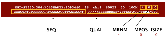
SAM/BAM format

The SAM file, is a tab-delimited text file that contains information for each individual read and its alignment to the genome. While we do not have time to go into detail about the features of the SAM format, the paper by Heng Li et al. provides a lot more detail on the specification.

The compressed binary version of SAM is called a BAM file. We use this version to reduce size and to allow for indexing, which enables efficient random access of the data contained within the file.

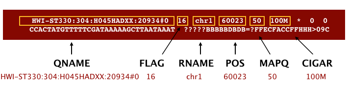
The file begins with a header, which is optional. The header is used to describe the source of data, reference sequence, method of alignment, etc., this will change depending on the aligner being used. Following the header is the alignment section. Each line that follows corresponds to alignment information for a single read. Each alignment line has 11 mandatory fields for essential mapping information and a variable number of other fields for aligner specific information. An example entry from a SAM file is displayed below with the different fields highlighted.

We will convert the SAM file to BAM format using the samtools program with the view command (yeah, it’s a funny name for the conversion process) and tell this command that the input is in SAM format (-S) and to output BAM format (-b). First we’ll need to load the samtools module.

BASH

$ module load samtools-1.10-gcc-9.3.0-flukja5
$ cd ~/1_project
$ samtools view -S -b results/sam/V1_S1_L001_ds_trim_align.sam > results/bam/V1_S1_L001_ds_trim_align.bam

This process can take a little while! You can speed it up using the -@ option to allocate additional CPUs to the task (e.g., try -@ 4).

Sort BAM file by coordinates

Next we sort the BAM file using the sort command from samtools. -o tells the command where to write the output. Notice that we are saving the file back into the same name, so the previous unsorted file will be overwritten by the sorted one. This saves us some space, but might be a bad idea if want to know which files are sorted and which are not. In that case, you would give the output a different name.

BASH

$ samtools sort -o results/bam/V1_S1_L001_ds_trim_align.bam results/bam/V1_S1_L001_ds_trim_align.bam

Our files are pretty small, so we will not see this output. If you run the workflow with larger files, you might see something like this:

OUTPUT

[bam_sort_core] merging from 2 files...

SAM/BAM files can be sorted in multiple ways, e.g. by location of alignment on the chromosome, by read name, etc. It is important to be aware that different alignment tools will output differently sorted SAM/BAM, and different downstream tools require differently sorted alignment files as input. The default, which we are using here, is to sort by the alignment coordinates in the reference genome.

You can use samtools to learn more about this sorted bam file as well.

BASH

samtools flagstat results/bam/V1_S1_L001_ds_trim_align.bam

This will give you the following statistics about your sorted bam file:

OUTPUT

2280568 + 0 in total (QC-passed reads + QC-failed reads)
357208 + 0 secondary
0 + 0 supplementary
0 + 0 duplicates
1422795 + 0 mapped (62.39% : N/A)
1923360 + 0 paired in sequencing
961680 + 0 read1
961680 + 0 read2
1022006 + 0 properly paired (53.14% : N/A)
1039730 + 0 with itself and mate mapped
25857 + 0 singletons (1.34% : N/A)
15468 + 0 with mate mapped to a different chr
11429 + 0 with mate mapped to a different chr (mapQ>=5)

Exercise

What do these different values mean? You might think to start with samtools flagstat --help, but that just gives you the options for the command. What could you do to find out more?

Show me the solution

There are two common approaches to this kind of challenge:

1. It is a good idea to start with the full documentation or manual, which is usually available online. The manual for samtools and associated programs is from HTSlib here, but it is not immediately clear how to find the information on the flagstat command. You can find the specific manual page here after a little poking around.

2. If the manual doesn’t help you, you can also try searching the internet with your question. Good search terms are specific and clear. In this case, you could try “samtools flagstat output”. The first hit (at least for me) is the manual, but the second is a forum post on Biostars that might be helpful!

If these two approaches don’t work, you can also talk to someone else working on similar problems, make your own post on a help forum, or reach out to the people who made the program (see the attribution or citation)!

In order for us to do some of our next steps, we will need to index the BAM file using samtools:

BASH

$ samtools index results/bam/V1_S1_L001_ds_trim_align.bam

This generates another file with the same name but a new extension, .bai (bam index).

Feature (read) counting

---

Read counting is calculating the number of reads for a particular sample that align to the reference at a given position, possibly at a gene or part of a gene. Similar to other steps in this workflow, there are a number of tools available for read counting. In this workshop we will be using the featureCounts program within the subread package. Note: a package is a word we use to describe a collection of programs or scripts.

Our final output here will be a matrix with genes or other genomic features as rows and samples as columns, with the number of reads aligned to that feature in that sample in each cell.

First, let’s find and load the module.

BASH

$ module avail subread

OUTPUT

-------------------------- /share/apps/modulefiles/modules ---------------------------
   subread-2.0.2-gcc-10.2.0

Use "module spider" to find all possible modules and extensions.
Use "module keyword key1 key2 ..." to search for all possible modules matching any of
the "keys".

Okay, let’s load the module and run it on our sorted, indexed bam file. We need to give featureCounts an annotation file after the -a flag. Annotation files store where different genomic features like genes or parts of genes are start and end in the genome. For this project, our annotation file is our gene transfer format (.gtf) genome file. We will also give it the output file name after -o, tell it to use 24 threads (-T 24), that the input is paired end (-p), and to only count read pairs with both ends aligned (-B) to the same strand of the same chromosome (-C). Remember that we can learn more about these options with the manual or with featureCounts --help. Finally, we tell featureCounts where to find the input file or files.

BASH

$ module load subread-2.0.2-gcc-10.2.0
$ featureCounts -a data/genome/Homo_sapiens.GRCh38.111.gtf -o results/counts/V1_S1_L001_counts.txt -T 24 -p -B -C results/bam/V1_S1_L001_ds_trim_align.bam

You should see output that looks like this:

OUTPUT

        ==========     _____ _    _ ____  _____  ______          _____
        =====         / ____| |  | |  _ \|  __ \|  ____|   /\   |  __ \
          =====      | (___ | |  | | |_) | |__) | |__     /  \  | |  | |
            ====      \___ \| |  | |  _ <|  _  /|  __|   / /\ \ | |  | |
              ====    ____) | |__| | |_) | | \ \| |____ / ____ \| |__| |
        ==========   |_____/ \____/|____/|_|  \_\______/_/    \_\_____/
	  v2.0.2

//========================== featureCounts setting ===========================\\
||                                                                            ||
||             Input files : 1 BAM file                                       ||
||                                                                            ||
||                           V1_S1_L001_ds_trim_align.bam                     ||
||                                                                            ||
||             Output file : V1_S1_L001_counts.txt                            ||
||                 Summary : V1_S1_L001_counts.txt.summary                    ||
||              Paired-end : yes                                              ||
||        Count read pairs : no                                               ||
||              Annotation : Homo_sapiens.GRCh38.111.gtf (GTF)                ||
||      Dir for temp files : results                                          ||
||                                                                            ||
||                 Threads : 24                                               ||
||                   Level : meta-feature level                               ||
||      Multimapping reads : not counted                                      ||
|| Multi-overlapping reads : not counted                                      ||
||   Min overlapping bases : 1                                                ||
||                                                                            ||
\\============================================================================//

//================================= Running ==================================\\
||                                                                            ||
|| Load annotation file Homo_sapiens.GRCh38.111.gtf ...                       ||
||    Features : 1650905                                                      ||
||    Meta-features : 63241                                                   ||
||    Chromosomes/contigs : 47                                                ||
||                                                                            ||
|| Process BAM file V1_S1_L001_ds_trim_align.bam...                           ||
||    Paired-end reads are included.                                          ||
||    The reads are assigned on the single-end mode.                          ||
||    Total alignments : 2280568                                              ||
||    Successfully assigned alignments : 709130 (31.1%)                       ||
||    Running time : 0.01 minutes                                             ||
||                                                                            ||
|| Write the final count table.                                               ||
|| Write the read assignment summary.                                         ||
||                                                                            ||
|| Summary of counting results can be found in file "results/V1_S1_L001_coun  ||
|| ts.txt.summary"                                                            ||
||                                                                            ||
\\============================================================================//

And if you look in the results/counts/ directory, you can see two new files:

BASH

$ ls results/counts

OUTPUT

V1_S1_L001_counts.txt  V1_S1_L001_counts.txt.summary

If we look at the summary file, we can learn a bit more about how well this sample performed. You might want to look up what the different values mean.

BASH

$ less results/counts/V1_S1_L001_counts.txt.summary

OUTPUT

Status  results/bam/V1_S1_L001_ds_trim_align.bam
Assigned        709130
Unassigned_Unmapped     857773
Unassigned_Read_Type    0
Unassigned_Singleton    0
Unassigned_MappingQuality       0
Unassigned_Chimera      0
Unassigned_FragmentLength       0
Unassigned_Duplicate    0
Unassigned_MultiMapping 509021
Unassigned_Secondary    0
Unassigned_NonSplit     0
Unassigned_NoFeatures   62313
Unassigned_Overlapping_Length   0
Unassigned_Ambiguity    142331

Exercise

Now that we have run through our workflow for a single sample, we want to repeat this workflow for our other samples. However, we do not want to type each of these individual steps again each time. That would be very time consuming and error-prone, and would become impossible as we gathered more and more samples. Luckily, we already know the tools we need to use to automate this workflow and run it on as many files as we want using a single line of code. Those tools are: wildcards, for loops, bash scripts, and job submission with slurm. Your challenge is to do this!

Hint: Remember that featureCounts can take multiple bam files as input, and will put them altogether in a single count file.

Show me the solution

Your solution can take many forms, but you will know you have solved it when you have a single count and count summary file in results/counts/ for all three samples, after running one or more sbatch scripts!

Once you have all the samples aligned, compressed to bam, sorted, indexed, and feature counted, we’re ready to do some data science!

Installing software

It is worth noting that all of the software we are using for this workshop has been pre-installed on our remote server. Not every program that you might need to use will be installed, however. You might need to install the software, or to ask the people in charge of your remote server to install it for you. It’s a good idea to find out how your specific remote server managers prefer that you do this. There might be a wiki or help page for the computer cluster, or you might need to email someone. Chimera is managed by Jeff Dusenberry, the director of research computing at UMass Boston. You can email him or another IT professional at It-rc@umb.edu. There is also a short informational page about applications (programs) on chimera.

Key Points

• Bioinformatic command line tools are collections of commands that can be used to carry out bioinformatic analyses.
• To use most powerful bioinformatic tools, you will need to use the command line.
• There are many different file formats for storing genomics data. It is important to understand what type of information is contained in each file, and how it was derived.

Content from Analyzing Read Count Data

---

Last updated on 2024-08-21 | Edit this page

Estimated time: 45 minutes

Overview

Questions

• How do we statistically identify and visualize differential gene expression patterns?

Objectives

• Normalize and process read counts for downstream analysis.
• Use a prepared R script on the command line to generate analysis results.

Exercise

It is a good idea to add comments to your code so that you (or a collaborator) can make sense of what you did later. Look through your existing scripts. Discuss with a neighbor where you should add comments. Add comments (anything following a # character will be interpreted as a comment, bash will not try to run these comments as code).

Analyzing Feature Count Data

---

We made it to the end of this analysis pipeline! Now we have read count data for samples across the human genome feature like genes and parts of genes. After this, our analyses become less like a pipeline and more like statistics. We’re going to think more about how to analyze count data in this episode. First, a quick review of the steps we took and our reasoning for those choices.

Central Data Analysis Themes

• Mapping to Transcriptome: No novel transcript discovery
• Mapping to Genome
• De Novo Assembly: When no reference genome is available

Sequencing Platforms

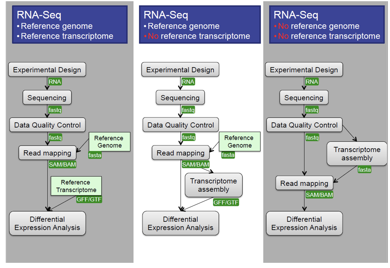
Data Quality Control

We learned and applied these approaches in previous episodes.

Quality Assessment: Evaluate read library quality using tools like FastQC.

Quality Control

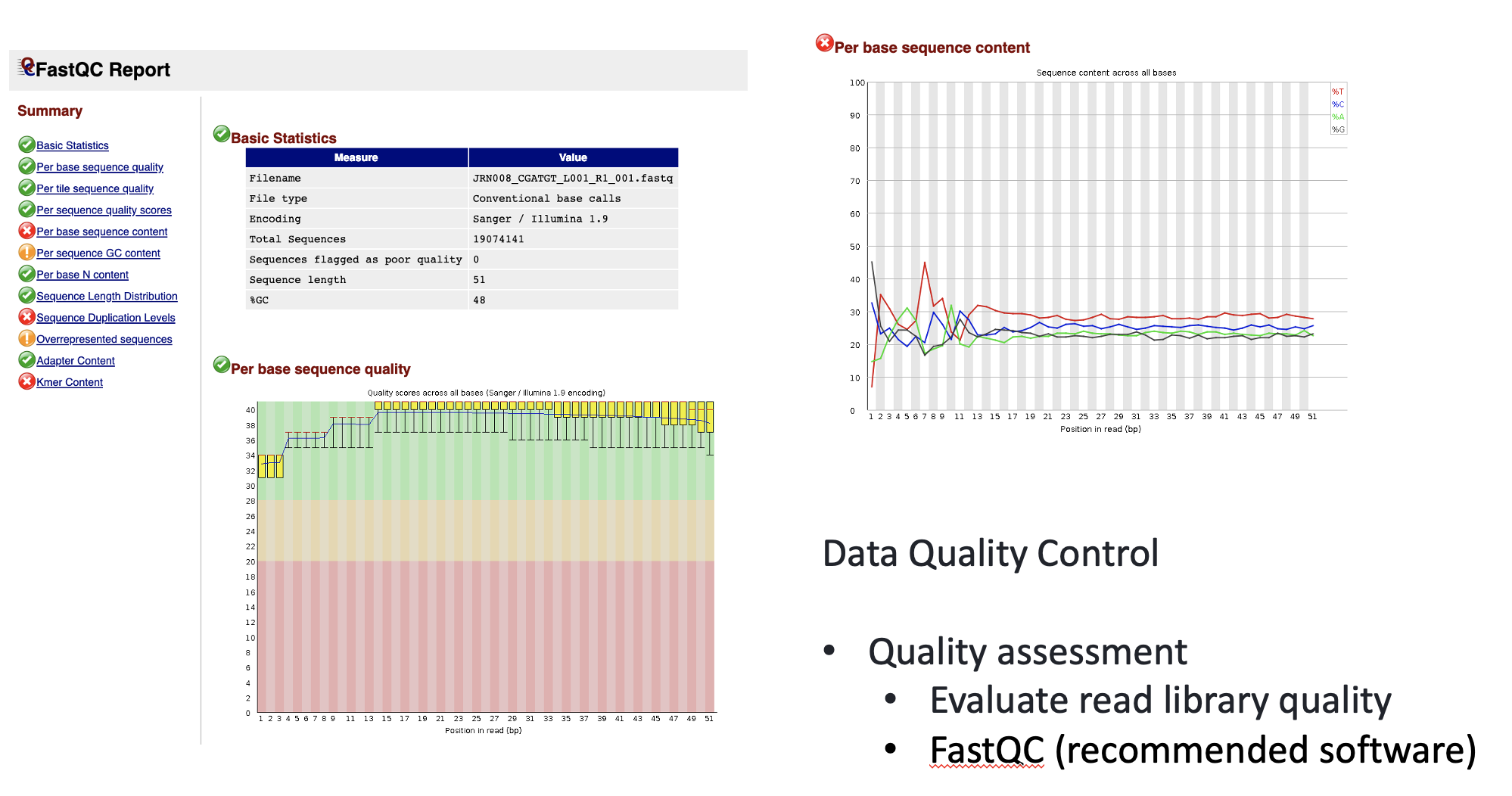
Filtering and Trimming: - Trim low-quality bases and adapter contamination from reads. - Filter out low-quality reads and sequence repeats. - Remove short reads (for example, <25 bp).

Trimming

Alignment to Reference Genome

Alignment Protocols

• Short Sequence Aligners: BWA, Bowtie2
• RNA-Seq Specific: TopHat2, HISAT2, STAR

Alignment Workflow

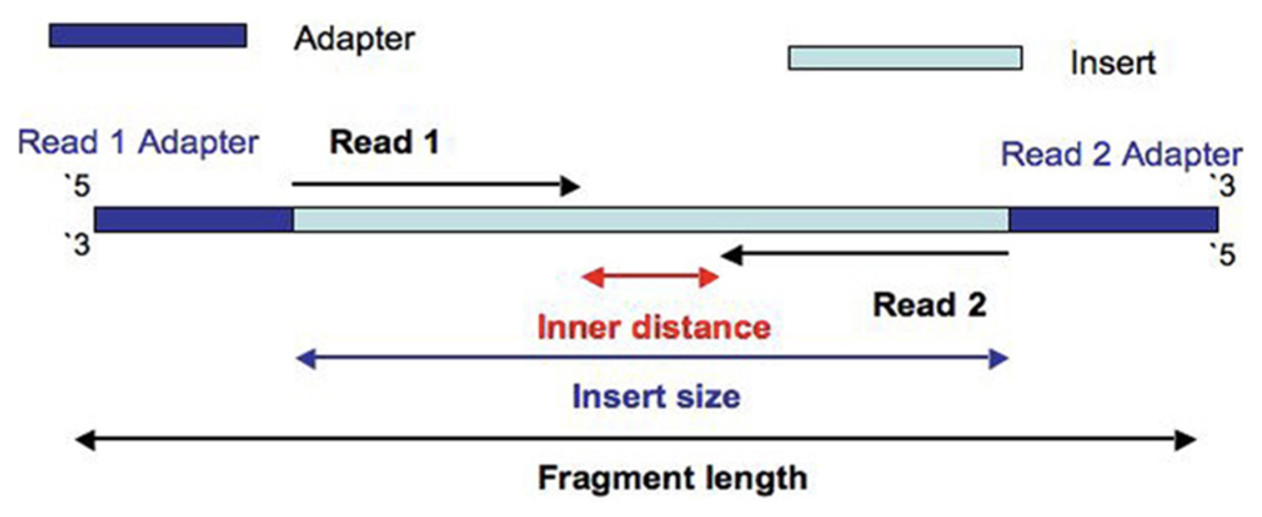
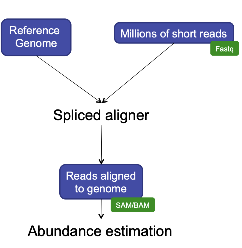
HISAT2

We used this program for alignment because it has a short processing time, simple quantification method (read counts), and differential analysis has low false positives.

hisat2 Alignment Workflow

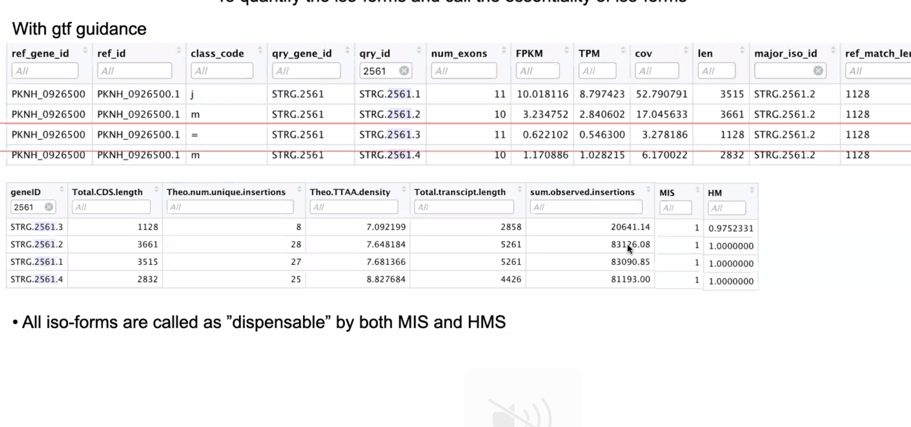
HISAT2 is splicing aware

• Unlike DNA alignment, RNA-Seq reads may span across introns due to differences in splicing.
• Usually 35% of reads will span multiple exons
• HISAT2 is a splice aware aligner (based on Bowtie2, uses many genome index files)
• Runs significantly faster than Bowtie2 and uses ~8Gb of memory
• On 100 million reads, it takes about 1 hour to finish the alignment process.

Splice-aware alignment

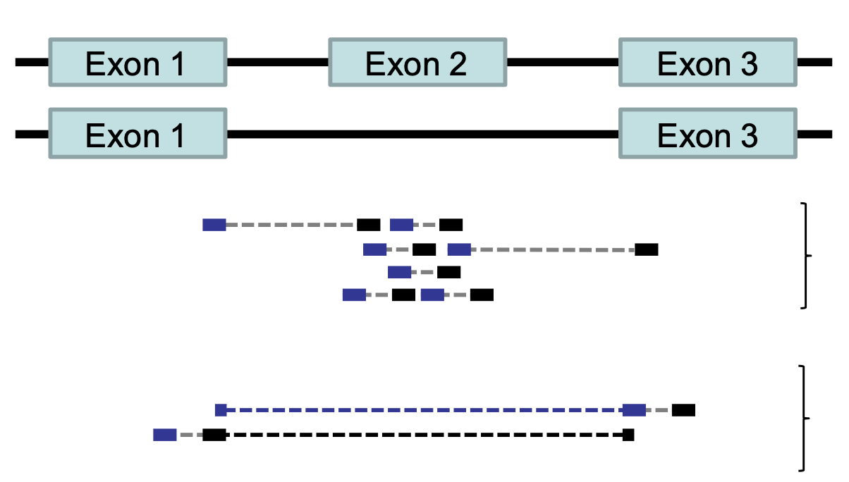
RNA-Seq: HISAT2 output

hisat2 --threads 20 -x ../grch38/genome --known-splicesite-infile ../HS_hisat2_known_splice_sites.txt -1 ../trim_galore_out/JRN008_CGATGT_L001_R1_001_val_1.fq -2 ../trim_galore_out/JRN008_CGATGT_L001_R2_001_val_2.fq -S ./hisat2_out/JRN008_CGATGT_L001.sam

• Output:
  • SAM / BAM alignment files
  • Software: SAMtoold
  • Contain statistics:
  • Uniquely mapped reads
  • Reads with multiple alignment
  • Unmapped reads
  • Properly paired reads

Typical hisat2 output (sam formatted)

featureCounts

• featureCounts takes as input SAM/BAM files and an annotation file as input.
• It outputs numbers of reads assigned to features (or meta-features).
• It also outputs stat info for the overall summarization results.

featureCounts -T 5 -t exon -g gene_id -a ../annotation.gtf -o ../counts.txt ./hisat2_out/JRN008_CGATGT_L001.sam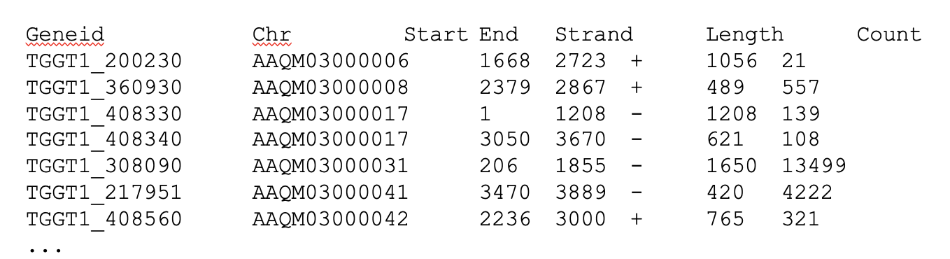

Table of the number of counts of each gene

edgeR

Differential Expression Analysis

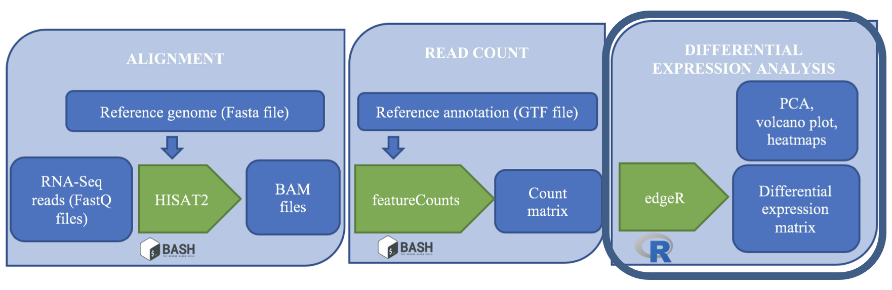
edgeR is a Bioconductor R package that implements statistical methods based on generalized linear models (glms), suitable for multi-factor experiments of any complexity. edgeR can be applied to differential expression at the gene, exon, transcript or tag level for any design.

Code Example (note that this written in the language R): design <- model.matrix(~treatment) CPM <- cpm(counts[2:ncol(counts)]) y <- DGEList(counts=x, group=treatment) y <- calcNormFactors(y) fit <- glmQLFit(new.y, new.design, robust=TRUE) qlf <- glmQLFTest(fit) tt <- topTags(qlf) summary(decideTests(qlf)) plotMD(qlf)

Example edgeR output

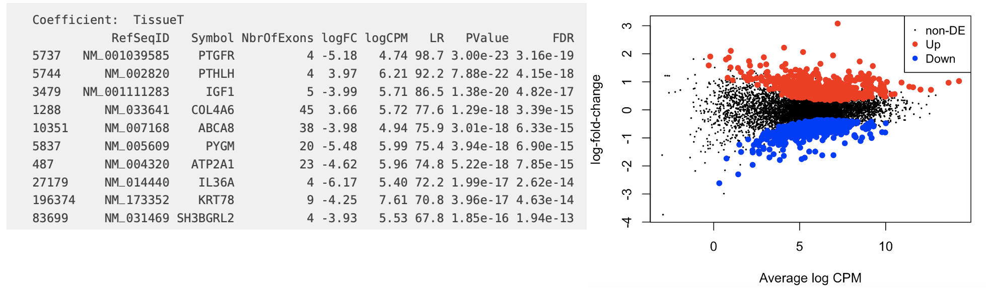
Key Points

• Our downstream steps take us into new territory: the R language.
• You can run R scripts on the command line.